lupine-publishers-mams - Tumblr blog

lupine-publishers-mams · 3 years

Text

Lupine Publishers| What is Quantum Computing and How it Works, Artificial Intelligence Driven by Quantum Computing

Lupine Publishers| Modern Approaches on Material Science

Abstract

Companies such as Intel as a pioneer in chip design for computing are pushing the edge of computing from its present Classical Computing generation to the next generation of Quantum Computing. Along the side of Intel corporation, companies such as IBM, Microsoft, and Google are also playing in this domain. The race is on to build the world’s first meaningful quantum computer-one that can deliver the technology’s long-promised ability to help scientists do things like develop miraculous new materials, encrypt data with near-perfect security and accurately predict how Earth’s climate will change. Such a machine is likely more than a decade away, but IBM, Microsoft, Google, Intel, and other tech heavyweights breathlessly tout each tiny, incremental step along the way. Most of these milestones involve packing more quantum bits, or qubits-the basic unit of information in a quantum computer-onto a processor chip ever. But the path to quantum computing involves far more than wrangling subatomic particles. Such computing capabilities are opening a new area into dealing with the massive sheer volume of structured and unstructured data in the form of Big Data, is an excellent augmentation to Artificial Intelligence (AI) and would allow it to thrive to its next generation of Super Artificial Intelligence (SAI) in the near-term time frame.

Keywords: Quantum Computing and Computer, Classical Computing and Computer, Artificial Intelligence, Machine Learning, Deep Learning, Fuzzy Logic, Resilience System, Forecasting and Related Paradigm, Big Data, Commercial and Urban Demand for Electricity

Introduction

Quantum Computing (QC) is designed and structured around the usage of Quantum Mechanical (QM) concepts and phenomena such as superposition and entanglement to perform computation. Computers that perform quantum computation are known as Quantum Computers[1-5].Note that the superposition from a quantum point of view is a fundamental principle of quantum mechanics. The Quantum Superposition (QS) states that, much like waves in Classical Mechanics (CM) or Classical Physics (CP), any two or more quantum states can be added together (“superposed”), and the result will be another valid quantum state; and conversely, that every quantum state can be represented as a sum of two or more other distinct countries.Mathematically, it refers to a property of solutions to the both Schrödinger Time-Dependent and Time-Independent Wave Equations; since the Schrödinger equation is linear, any linear combination of solutions will also be a solution.An example of a physically observable manifestation of the wave nature of quantum systems is the interference peaks from an electron beam in a double-slit experiment, as illustrated in (Figure 1).The pattern is very similar to the one obtained by the diffraction of classical waves. [6]. Quantum computers are believed to be able to solve some computational issues, such as integer factorization, which underlies RSA encryption [7], significantly faster than classical computers. The study of quantum computing is a subfield of quantum information science.

Figure 1: Double-Slit Experiment Setup.

Historically, Classical Computer (CC) technology, as we know them from the past few decades to present, has involved a sequence of changes from one type of physical realization to another, and they have been evolved from main-frame of the old generation to generation of macro-computer. Now, these days, pretty much everyone owns a minicomputer in the form of a laptop, and you find these generations of computers in everyone’s house as part of their household. These mini-computers, Cemeterial Processing Units (CPUs), are based on transistors that are architected around Positive-Negative-Positive (PNP) junction.From gear to relays to valves to transistors to integrated circuits and so on we need automation and consequently augmentation of computer of some sort Today’s advanced lithographic techniques at below sub-micron innovative structure augmenting techniques such as Physical Vapor Deposition (PVD), Chemical Vapor Deposition (CVD), and Chemical Mechanical Polishing (CMP) can create chips with a feature only a fraction of micron wide. Fabricator and manufacturer these chips are pushing them to yield even smaller parts and inevitably reach a point where logic gates are so small that they are made out of only a handful of atoms size, as it is depicted in (Figure 2).

Figure 2: Today’s Chip Fabrication.

It worth mentioning that the size of the chip going way beyond sub-micron technology is limited by the wavelength of the light that is used in the lithographic technique. On the atomic scale, matter obeys the rules of Quantum Mechanics (QM), which are quite different from Classical Mechanics (CM) or Physics Rules that determine the properties of conventional logic gates. Thus, if computers are to become smaller in the future, new, quantum technology must replace or supplement what we have new as a traditional way of computing.The point is, however, that quantum technology can offer much more than cramming more and more bits onto silicon CPU chip and multiplying the clock-speed of these traditional microprocessors. It can support an entirely new kind of computation with qualitatively new algorithms based on quantum principles! In a nutshell, in Quantum Computing, we deal with Qubits, while in Classical Computing, we deal with bits of information; thus, we need to understand “What Are Qubits?” and how it is defined, which we have presented this matter further down.Next generation of tomorrow’s computer is working based on where “Quantum Bits Compressed for the First Time.” The physicist has now shown how to encode three quantum bits, the kind of data that might be used in this new generation of computer, by just using two photons.Of course, a quantum computer is more than just its processor. These next-generation systems will also need new algorithms, software, interconnects, and several other yet-tobe- invented technologies specifically designed to take advantage of the system’s tremendous processing power-as well as allow the computer’s results to be shared or stored.

Intel introduced a 49-qubit processor code-named “Tangle Lake.” A few years ago, the company created a virtual-testing environment for quantum-computing software; it leverages the powerful “Stampede” supercomputer at The University of Texas at Austin to simulate up to a 42-qubit processor. To understand how to write software for quantum computers, however, they will need to be able to simulate hundreds or even thousands of qubits.Note that: Stampede was one of the most potent and significant supercomputers in the U.S. for open science research. Able to perform nearly ten quadrillion operations per second, Stampede offered opportunities for computational science and technology, ranging from highly parallel algorithms, highthroughput computing, scalable visualization, and next-generation programming languages, as illustrated in (Figure3) here. [8]This Dell PowerEdge cluster equipped with Intel Xeon Phi coprocessors pushed the envelope of computational capabilities, enabling breakthroughs never before imagined. Stampede was funded by the National Science Foundation (NSF) through award ACI-1134872.

Figure 3: Array of Stampede Structure.

Stampede was upgraded in 2016 with additional compute nodes built around the second generation of the Intel Xeon Phi many-core, x86 architecture, known as Knights Landing. The new Xeon Phi’s function as the primary processors in the new system. The upgrade ranked #116 on the June 2016 Top 500 and was the only KNL system on the list.Note that: Knights Landing (KNL) is 2nd Generation of Intel® Xeon Phi™ Processor

What Are Qubits?

A qubit can represent a 0 and 1 at the same time, a uniquely quantum phenomenon known in physics as a superposition. This lets qubits conduct vast numbers of calculations at once, massively increasing computing speed and capacity. But there are different types of qubits, and not all are created equal. In a programmable silicon quantum chip, for example, whether a bit is 1 or a 0 depends on the direction its electron is spinning. Yet all qubits are notoriously fragile, with some requiring temperatures of about 20 millikelvins-250 times colder than deep space-to remain stable. From a physical point of view, a bit is a physical system, which can be prepared in one of the two different states representing two logical values: based on No or Yes, False or True, or simply 0 or 1.Quantum bits, called qubits, are implemented using quantum mechanical two-state systems, as we stated above. These are not confined to their two basic states but can also exist in superposition. This means that the qubit is both in state 0 and state 1, as illustrated in (Figure 4).Any classical register composed of three bits can store in a given moment, only one out of eight different numbers, as illustrated in (Figure 5). A quantum register composed of three qubits can store in a given momentum of time all eight numbers in a quantum superposition, again as illustrated in (Figure5).Once the register is prepared in a superposition of different numbers, one would be able to perform operations on all of them, as demonstrated in (Figure 6)here. Thus, quantum computers can perform many different calculations in parallel. In other words, a system with N qubits can perform 2N calculations at once!

Figure 4: Logical Value Representation.

Figure 5: Classical Vs. Quantum Register.

Figure 6: Quantum Processor Demonstration.

This has impact on the execution time and memory required in the process of computation and determines the efficiency of algorithms. In summary, A memory consisting of N bits of information has 2N possible states. A vector representing all memory states thus has 2N entries (one for each state). This vector is viewed as a probability vector and represents the fact that the memory is to be found in a particular state level. [9]In the classical view, one entry would have a value of 1 (i.e., a 100% probability of being in this state), and all other entries would be zero. In quantum mechanics, probability vectors are generalized to density operators [10]. This is the technically rigorous mathematical foundation for quantum logic gates [11], but the intermediate quantum state vector formalism is usually introduced first because it is conceptually simpler.However, one question arises about Qubits and that is “Why are qubits so fragile?” and here is what we can say.The reality is that the coins, or qubits, eventually stop spinning and collapse into a particular state, whether it’s heads or tails. The goal with quantum computing is to keep them spinning in the superposition of multiple Furthermore, expanding on Quantum Operations, and we stated concerning this operation, the prevailing model of Quantum Computation (QC) describes the computation in terms of a network of Quantum Logic Gates[12].

Bear in mind that, a quantum computing and specifically the quantum circuit model of computation, a quantum logic gate (or merely quantum gate) is a primary quantum circuit operating on a small number of qubits. They are the building blocks of quantum circuits like classical logic gates are for conventional digital circuits [13].States for a long time. Imagine I have a coin spinning on a table, and someone is shaking that table. That might cause the coin to fall over faster. Noise, temperature change, an electrical fluctuation or vibration-all of these things can disturb a qubit’s operation and cause it to lose its data. One way to stabilize certain types of qubits is to keep them very cold. Our qubits operate in a dilution refrigerator that’s about the size of a 55-gallon drum and use a particular isotope of helium to cool them a fraction of a degree above absolute zero (roughly –273 degrees Celsius) [7].There are probably no less than six or seven different types of qubits, and probably three or four of them are being actively considered for use in quantum computing. The differences are in how you manipulate the qubits, and how you get them to talk to one another. You need two qubits to talk to one another to do large “entangled” calculations, and different qubit types have different ways of entangling.Another approach uses the oscillating charges of trapped ions-held in place in a vacuum chamber by laser beams-to function as qubits. Intel is not developing trapped ion systems because they require a deep knowledge of lasers and optics, which is not necessarily suited to our strengths.Furthermore, quantum computers being built by Google, IBM, and others. Another approach uses the oscillating charges of trapped ions-held in place in a vacuum chamber by laser beams-to function as qubits. Intel is not developing trapped ion systems because they require a deep knowledge of lasers and optics, which is not necessarily suited to our strengths.

How Powerful Are Quantum Computers?

For an algorithm to be efficient, the time it will take to execute the algorithm must increase not faster than a Polynomial Function of the size of the input. For example, let us think about the input size as the total number of bits needed to specify the input to the problem, as demonstrated in(Figure 7). The number of bits required to encode the number we want to factorize is an example of this scenario.If the best algorithm we know for a particular problem has the execution time, which can be viewed as a function of the size of the input, bounded by a polynomial, then we say that the problem belongs to Class P, as it is shown in (Figure 7).Problems outside class P are known as hard problems. Thus, we say, for example, that multiplication is in P, whereas factorization is not in P. “Hard” in this case does not mean that it is “impossible to solve” or “noncomputable”. It means that the physical resources needed to factor a large number scale up such that, for all practical purposes, it can be regarded as intractable.However, some quantum algorithms can turn hard mathematical problems into easy ones – factoring being the most striking example as far as we are concerned so far. Such a scenario can be seen in cryptographic technology to be able to decipher a code of cryptic streams or communications. One can see a huge application of it in Rivest, Shamir, and Adelman (RSA) Data Security[8].

Figure 7: Polynomial Function.

The difficulty of factorization underpins the security of what are currently the most trusted methods of public-key encryption, in particular of the RSA system, which is often used to protect electronic bank account, as depicted in (Figure 8).Once a quantum factorization engine, which is a special-purpose quantum computer for a factorizing large number, is built, all such cryptographic systems will become insecure, and they will be wide-open for smart malware to pass through the gate of cybersecurity wall of the system under the attack by this malware.The potential use of quantum factoring for code-breaking purposes has raised the apparent suggestion of building a Quantum Computer (QC), however this not the only application QC. With signs of progress in the utilization of Artificial Intelligence (AI) in the recent decade and pushing toward Super Artificial Intelligence (SAI) to deal with massive sheer of data at Big Data (BD) volume, a need for Quantum Computing versus Classical Computing is felt by the today’s market standard.A supervised AI or SAI with an integrated element of Machine Learning (ML) and Deep Learning (DL) allows us to prosses all of the historical data by comparing them with a collection of incoming data via DL and ML to collect the right information for a proper decision making of the ongoing day-to-day operation and most importantly to be able to forecast future as a paradigm model [14-17].

Figure 8: RSA Data Security Key.

The impact of quantum computing on developing a better artificial intelligence and its next-generation super artificial intelligence can be seen as ongoing technology efforts by scientists and engineers as a common denominator.Typically, the first quantum algorithms that get proposed are for security (such as cryptography) or chemistry and materials modeling. These are problems that are essentially intractable with conventional computers. That said, there are a host of papers as well as start-up companies and university groups working on things like machine learning and AI using quantum computers. Given the time frame for AI development, “I would expect conventional chips optimized specifically for AI algorithms to have more of an impact on the technology than quantum chips,” says Jim Clarke, Intel’s Head of Quantum Computing. Still, AI is undoubtedly a fair game for quantum computing.

How to Build Quantum Computers?

In principle, engines know, how to build a Quantum Computer; we start with simple quantum logic gates as it was described in general previously and connect them up into quantum networks [9] as depicted herein (Figure 9).A Quantum Logic Gate (QLG), like its cousin Classical Logic Gate (CLG), is a straightforward computing device that performs one elementary quantum operation around qubit, usually on two qubits, in a given time. Of course, quantum logic gates differ from their classical counterparts in that they can create and perform operations on quantum superposition as we stated before.As the number of quantum gates in a network increases, we quickly run into some serious practical problems. The more interacting qubits are involved, the harder it tends to be engineering the interaction that would display the quantum properties.The more components there are, the more likely it is that quantum information will spread outside the quantum computer and be lost into the environment, thus spoiling the computation. This process is called decoherence. Therefore, our task is to engineer a sub-microscopic system in which qubits affect each other but not the environment.This usually means isolating the system from its environment as interactions with the external world cause the system to decohere. However, other sources of decoherence also exist. Examples include the quantum gates, and the lattice vibrations and background thermonuclear spin of the physical system used to implement the qubits. Decoherence is irreversible, as it is effectively non-unitary, and is usually something that should be highly controlled, if not avoided.

Figure 9: A Simple Quantum Logic Gates.

Considering such constraint, then it is clear which technology will support quantum computation going forward in the future of this technology. Today simple quantum logic gates involving two qubits, as we said, are being realized and recognized in laboratories as stepping forward. Current experiments range from trapped ions via atoms in an array of potential wells created by a pattern of the crossed laser beam to electrons in semiconductors. See (Figure 10) However, the technology of the next decade should bring control over several qubits and, without any doubt, we shall already begin to benefit from our new way of harnessing nature.There are several models of quantum computing, including the quantum circuit model, quantum Turing machine, adiabatic quantum computer, one-way quantum computer, and various quantum cellular automata. The most widely used model is the quantum circuit. Quantum circuits are based on the quantum bit, or “qubit”, which is somewhat analogous to the bit in classical computation. Qubits can be in a 1 or 0 quantum state, or they can be in a superposition of the 1 and 0 states. However, when qubits are measured, the result is always either a 0 or a 1; the probabilities of these two outcomes depend on the quantum state that they were in immediately before the measurement. Computation is performed by manipulating qubits with quantum logic gates, which are somewhat analogous to classical logic gates[9].There are currently two main approaches to physically implementing a quantum computer: analog and digital. Analog methods are further divided into the quantum simulation, quantum annealing, and adiabatic quantum computation. Digital quantum computers use quantum logic gates to do computation. Both approaches use quantum bits or qubits[10] There are currently several significant obstacles in the way of constructing useful quantum computers. In particular, it is difficult to maintain the quantum states of qubits as they are prone to quantum decoherence, and quantum computers require significant error correction as they are far more prone to errors than classical computers[10].

Figure 10: Patten of Crossed Laser Beam.

Conclusion

The race is on to build the world’s first meaningful quantum computer-one that can deliver the technology’s long-promised ability to help scientists do things like develop miraculous new materials, encrypt data with near-perfect security and accurately predict how Earth’s climate will change. Such a machine is likely more than a decade away, but IBM, Microsoft, Google, Intel, and other tech heavyweights breathlessly tout each tiny, incremental step along the way. Most of these milestones involve packing more quantum bits, or qubits-the basic unit of information in a quantum computer-onto a processor chip ever. But the path to quantum computing involves far more than wrangling subatomic particles. However, the question of “When will we see working Quantum Computer solving real-world problems?” remains to be answered. The first transistor was introduced in 1947. The first integrated circuit followed in 1958. Intel’s first microprocessor-which had only about 2,500 transistors-didn’t arrive until 1971. Each of those milestones was more than a decade apart. People think quantum computers are just around the corner, but history shows these advances take time. If 10 years from now we have a quantum computer that has a few thousand qubits, that would undoubtedly change the world in the same way the first microprocessor did. We and others have been saying it’s ten years away. Some are saying it’s just three years away, and I would argue that they don’t have an understanding of how complex the technology is. At the end, it is worthy to say that “Any computational problem that can be solved by a classical computer can also, in principle, be solved by a quantum computer. Conversely, quantum computers obey the Church–Turing thesis; that is, any computational problem that can be solved by a quantum computer can also be solved by a classical computer. While this means that quantum computers provide no additional power over classical computers in terms of computability, they do, in theory, provide extra power when it comes to the time complexity of solving certain problems.Notably, quantum computers are believed to be able to quickly solve certain problems that no classical computer could solve in any feasible amount of time-a feat known as “quantum supremacy” [10].The study of the computational complexity of problems concerning quantum computers is known as quantum complexity theory.

For more Lupine Publishers Open Access Journals Please visit our website:

wt u have given that link add For more Modern Approaches on Material Science articles Please Click Here:

https://lupinepublishers.com/material-science-journal/

#lupinePublishers #lupine publishers group #open access journals #organic materials

0 notes

lupine-publishers-mams · 3 years

Text

Lupine Publishers| An Alternative Strategy for the Use of a Low-Cost, Age- Hard enable Fe-Si-Ti Steel for Automotive Application

Lupine Publishers| Modern Approaches On Material Science

Abstract

For High Strength Low Alloy (HSLA) steels or for age-hard enable steels (miraging) the strengthening by precipitation is done before forming operation to increase the yield stress as much as possible. In this publication the advantages of a hardening thermal treatment after forming operation are investigated in a low-cost age-hard enable steel Fe-Si-Ti consistent with automotive application.

Keywords: Age-hard enable, Precipitation, Forming, Ductility

Introduction

The high strength low alloy (HSLA) steels are a group of low carbon steels with small amounts of alloying elements (as Ti, V, Nb, etc.) to obtain a good combination of strength, toughness, and weldability [1-3]. By the addition of micro-alloying elements (less than 0.5 wt.%), HSLA steels are strengthened by grain refinement strengthening, solid solution strengthening and precipitation hardening [4-8]. Regarding automotive applications, the entire range of HSLA steels are suitable for structural components of cars, trucks, and trailers such as suspension systems, chassis, and reinforcement parts. HSLA steels offer good fatigue and impact strengths. Given these characteristics, this class of steels offers weight reduction for reinforcement and structural components [9-11]. Despite the interest of HSLA, the precipitation hardening is about 100MPa. So the new targets concerning the CO2 emission of vehicles push the steel-makers to develop Advanced High Strength Steels (Dual-Phase, Transformation Induced Plasticity) hardened by multiphase microstructures containing 10 to 100% of martensite [12] which offer a better combination between strength and ductility for an acceptable cost Let’s notice that the Ultimate Tensile Strength (UTS) increases more that the Yield Stress (YS). YS is crucial for anti-intrusive aspect during a crash [12]. In the other side, because there is no phase transformation in Aluminum, age-hardening by precipitation is widely used in Aluminium alloys hardened by various additive elements [see [13] for a review]. The volume fraction of precipitates is several percent’s, the hardening can be increased up to 400MPa, but the ductility decreases rapidly.

In steel, there is only miraging steels which are strengthened by a massive precipitation of a martensitic matrix [see [14] for a review]. Despite the impressive YS (up to 2.5GPa), the uniform elongation is less than 1%. Consequently, no forming operation is possible. In addition, the high contents of nickel (about 18%), of molybdenum and of cobalt make these steels very expensive and so they are never used in automotive industry. On the contrary, in the 60’s authors investigated other kind of steels suitable to be strongly hardened by massive intermetallic precipitation without extracost [15,16]. Among the different investigated system, the Fe-Si-Ti alloys are the most promising. This is the reason why a series of publications has been dedicated to this system in the 70’s by Jack&al. [17-19]. Unfortunately, hardness and compression behaviour have been only reported and a lot of discussions concerned the nature of the precipitates (Fe2Ti, FeSi, or Fe2SiTi) have been reported. More recently a systematic study of precipitation kinetics in a Fe-2.5%Si- 1%Ti alloy in the temperature range 723 K to 853 K (450°C to 580°C), combining complementary tools transmission electron microscopy (TEM), atom probe tomography (APT), and Small-Angle-Neutron Scattering (SANS)) have been carried out [20]. It has been shown that the Heusler phase Fe2SiTi dominates the precipitation process in the investigated time and temperature range, regardless of the details of the initial temperature history.

Figure 1: Summary of the different strategies for the use of precipitation hardened steels: The green arrow is the usual one, the orange is the strategy developed in this publication.

Considering that the ductility decreases regularly as a function of the hardening up to 1.2GPa and because it is targeted to obtain a steel suitable for deep drawing the strategy showed in (Figure 1). (orange arrow) has been investigated. The objective is to form a material as soft as possible and as ductile as possible and to obtain the hardening by a thermal treatment after forming. This publication presents the characterization of this way to manage the situation. It is noticed that as Si and Ti promote ferrite, there is no phase transformation whatever the thermal treatment. (Figure 1) Summary of the different strategies for the use of precipitation hardened steels: The green arrow is the usual one, the orange is the strategy developed in this publication.

Results

In order to assess for the first time in steel for automotive applications, the hardening have been chosen followed a thermal treatment at 500°C for two hours consistent with the kinetic determined by SANS [20]. As shown in (Figure 2). illustrating the tensile behavior of the steel consisting only in solid solution (i.e. only after recrystallization) is very ductile as for IF steels but with a higher yield stress due to solid solution hardening. After treatment and hardening of 300MPa is obtained with promising ductility. As shown in (Figure 3) the treatment has induced the expected massive precipitation of Fe2SiTi (3.8% weight percent with a radius of 4nm determined by TEM and SANS [20]). To assess the metallurgical route, the (Figure 4). shows that it is possible to severely bend the steel consisting only in solid solution without any defect up to an angle of 180°. Hardness trough the thickness has been measured before and after the thermal treatment (Figure 5). The value confirms the hardening by precipitation. It is noticed that tis precipitation hardening is not sensitive to the strain hardening induced by bending trough the thickness. Because the alloy is dedicated to automotive industry, the drawing must be investigated. This the reason why a cup obtained by deep drawing of 5cm diameter has been manufactured using the steel consisting in solid solution without any problem as illustrated in (Figure 6). It confirms the very high ductility before heat treatment. One another problem in automotive industry is the increase in spring-back with an increase in strength. In addition, it is very difficult to predict or to model this phenomenon. As shown in (Figure 7). this aspect has been studied by a standard test base the forming of a hat-shaped part. It is highlighted that the spring-back during the treatment is weak. That is probably because there is no phase transformation during precipitation and so no internal stresses.

Figure 2: Tensile curves before and after the ageing treatment.

Figure 3: TEM micrography showing the massive precipitation of Fe2SiTi after 2 hours at 500°C (the composition have been determined by APT [20]).

Figure 4: Fully bent specimen before heat treatment (bending angle of 180°).

Figure 5: Hardness measurement trough the thickness of the fully bent specimen (i.e. angle of 180°) before and after heat treatment.

Figure 6: Cup drawing before the hardening heat treatment (5cm diameter).

Figure 7: Evaluation of the effect of heat treatment on the spring-back.

Conclusion

For the first time in steel industry for automotive industry a low cost age-hard enable steel has been studied following a strategy based on forming operations before the heat treatment. The bending, the drawability and the spring-back have been investigated highlighting promising results. In addition, the alloy exhibits a cost acceptable for automotive industry. In the future crashworthiness and weldability should be assessed after heat treatment. One of the last advantages is that a lot of parts can be treated at the same time in a furnace usually dedicated to tempering treatment.

For more Lupine Publishers Open Access Journals Please visit our website:

wt u have given that link add For more Modern Approaches on Material Science articles Please Click Here:

https://lupinepublishers.com/material-science-journal/

#LupinePublishers #OpenaccessPublishers #lupinePublishersJournals #materialScience #compositeMaterials

0 notes

lupine-publishers-mams · 3 years

Text

Lupine Publishers| Monitoring Time-Progression of Structural, Magnetic Properties of Ni Nano Ferrite During Synthesis

Abstract

We present time-progression of structural, magnetic properties of NiFe2O4 nano ferrite during its synthesis via sol-gel auto combustion technique, monitored by x-ray diffraction XRD, and magnetic measurements. XRD patterns of the samples collected between 18-52 minutes shows the formation of the nano spinel phase (grain diameter: 15.4 nm-28.6 nm), presence of a-Fe2O3phase was also detected. Samples collected between 8-14 minutes show the amorphous nature of the samples. Time-progression studies show: a) sample taken after 20 minutes shows a sharp decrease of specific surface area (range between 39.01 m2/g to 72.73 m2/g), b) non-equilibrium cationic distribution for samples taken between 16-20 minutes with a continuous increase of Fe3+ ions population on B-site with simultaneous decrease of Ni2+ population, c) for samples taken after 22, 52 minutes, cationic distribution is close to its ideal value of (Fe3+) [Ni2+Fe3+], d) alteration of a degree of inversion (d), oxygen parameter (u), modification of A-O-B, A-O-A, B-O-B super-exchange interactions, e) ferrimagnetically aligned core, and spin disorder on the surface with a thickness between 1.9 nm to 3.6 nm, reducing the saturation magnetization (ranging between 11.7 - 25.5 Am2/kg), as compared to bulk Ni ferrite (55 Am2/kg), f) low squareness ratio values (0.15-0.22) shows the presence of multi-domain nanoparticles, with coercivity between 111-157 Oe.

Keywords: Time-evolution of properties; Sol-gel auto combustion synthesis; XRD; Nano Ni ferrite; Cationic distribution; Magnetic properties

Introduction

Spinel ferrites with general formula Me2+O.Fe3+2 O3, [Me: Divalent metal ion e.g. – Ni2+, Zn2+, Mg2+ Co2+ etc.], display face-centered cubic (fcc) structure, with two inter-penetrating sub-lattices: tetrahedrally coordinated (A site), octahedrally coordinated (B site) [1]. Nickel ferrite (NiFe2O4) has inverse spinel structure expressed as: (Fe3+) [Ni2+Fe3+] [1]. Allocation of cations on A, B site is crucial in determining properties of spinel ferrites [2,3], can be effectively used to achieve desired properties. Literature gives Ni ferrite synthesis using various methods including mechanical milling [4], coprecipitation [5], hydrothermal synthesis [6], sol-gel auto combustion method [7], showing the effect of the technique on structural, magnetic properties. Literature also reports real-time monitoring (in-situ studies) of properties [8,9], require special, sophisticated equipment, may not be available in all laboratories. Ex-situ monitoring of properties [10], describing the time-evolution of structural, magnetic properties, is a rather simple, more convenient way to perform experiments by utilizing standard laboratory equipment available in many laboratories. Ni ferrite is used in magnetic resonance imaging (MRI) agents [5], photocatalysis for water purification, antimicrobial activity [11], etc.) hence tuning its properties are preferred for improved efficiency.So, in this work, we present the time-development of structural, magnetic properties of NiFe2O4 nano ferrite during its synthesis via sol-gel auto combustion technique. Prepared samples are investigated via x-ray diffraction 'XRD,' vibration sample magnetometry, to get complimentary information on structural, magnetic properties.

Experimental Details

NiFe2O4 ferrite samples were synthesized by the sol-gel auto-combustion protocol, as described in detail in [12], by utilizing AR grade -nitrate/acetate-citrate precursors: Nickel acetate - Ni(CH₃CO₂)₂·4H₂O, Ferric nitrate (Fe(NO3)3.9H2O), Citric acid - C6H8O7]. The precursors were mixed in the stoichiometric ratio, were dissolved in 10 ml de-ionized water by keeping metal salts to fuel (citric acid) ratio as 1:1. At the same time, the solution pH was maintained at 7. Now the solution was heated at ~110 ̊C. As dry gel starts to form (taken as 0 minutes) small part of the sample is taken out from the reaction vessel (in an interval of 8, 10, 12, 14, 16, 18, 22, and 52 minutes), and were immediately ice-quenched to room temperature. Powder samples were used for Cu-K- X-ray diffraction 'XRD' measurements (Bruker D8 diffractometer), hysteresis loops by vibrating sample magnetometer. Full-profile XRD analysis was done by MAUD Rietveld refinement software [13] to obtain the lattice parameter (apex.). XRD analysis gives Scherrer's crystalline size D (calculated by the integral width of 311 peak, corrected for instrumental broadening), specific surface area (S), inversion parameter (d), oxygen parameter (u). XRD data was also analysed to get cationic distribution via Bertaut method [14], This provides cationic distribution by comparing experimental and computed intensity ratio of planes I(220)/I(400) and I(400)/I(422), susceptible to cationic distribution [12]. Cationic distribution was used to calculate theoretical or Néel magnetic moment at 0K (Ms(th)), theoretical lattice parameter (ath.), bond angles (θ1, θ2, θ3, θ4, θ5) as shown in [3]. Coercivity (Hc), saturation magnetization (Ms), remanence (Mr), squareness ratio (Mr/Ms) was obtained from hysteresis loops. (Figure 1) gives the schematic of sample synthesis and characterization.

Figure 1: Schematic of sample synthesis and characterization.

Results and Discussion

(Figure 2) (a) gives XRD-patterns of the studied NiFe2O4 samples collected after 18, 20, 22, and 52 minutes, confirm the formation of the spinel phase. XRD patterns also show the presence of a-Fe2O3 phase, ascribable to sample synthesis at a reasonably lower temperature (~110̊C), as reported in [15], while its disappearance is seen after higher sintering temperature. Figure 1(a) inset shows XRD patterns of samples collected after 8, 10, 12, 14 minutes show the amorphous nature of the samples. Only in the sample collected after 14 minutes, there is the start of spinel phase formation (indicated by a dotted circle). Illustrative Rietveld refined XRD pattern (Figure 2) b) of NiFe2O4 sample taken after 20 minutes also validates the cubic spinel ferrite phase formation. (Figure 2)(c) shows a variation of D (range between 15.4 nm to 28.6 nm) and S (range between 39.01 m2/g to 72.73 m2/g) for NiFe2O4 samples taken after 16, 18, 20 22, 52 minutes. A perusal of (Figure 2) (c) shows a well-known inverse relationship shown by the expression: [S = [6/(D ´rXRD)], where rXRDis x-ray density, as was also reported in[2]. (Figure 2) (c) shows that for samples taken after 22, 52 minutes, D sharply increases with concurrent reduction of S, is ascribable to significant changes in cationic distribution via migration of Ni2+ions to B site with simultaneous migration of Fe3+ ions on A site(as can be seen in Table 1). (Figure 2 )(c) inset display linear relation between d and u as was also observed earlier [3], shows that reduction of the degree of inversion (d) leads to a reduction of oxygen parameter (u), a measure of disorder in the studied system, is expected to affect the properties of the studied samples. Table 1 depicts the variation of experimental and theoretical lattice parameter (aexp., ath. ), inversion parameter (d), oxygen parameter (u), Cation distribution (for A, B site), and calculated, observed intensity ratios for I400/422, I220/400 plane for the studied samples. The observed variation of aexp. is consistent with changes in cationic distribution, and variation of the degree of inversion (d). Close agreement between observed, calculated aexp., ath. suggests that the computed cationic distribution agrees well with real distribution [16]. Close matching of calculated, observed intensity ratios for I400/422, I220/400 signifies an accurate cationic distribution among A, B site [17]. Cationic distribution illustrates that as we go from NiFe2O4 samples taken after 16, 18, and 20 minutes, the population of Fe3+ ions on B site increases from 1.2 to 1.5 with a concurrent decrease of Ni2+ ions from 0.80 to 0.50. For samples taken after 22, 52 minutes Fe3+ population on B site decreases, while Ni2+ ion population increases up to 0.98, which is close to the ideal inverse cationic distribution of (Fe3+) [Ni2+Fe3+] [1].

Figure 2: (a): XRD patterns of the studied NiFe2O4 samples taken after 16, 18, 20 22, 52 minutes showing the formation of the spinel phase. Inset: XRD patterns of the studied samples taken after 8, 10, 12, 14 minutes. (b): Illustrative Rietveld refined XRD pattern of NiFe2O4 sample taken after 20 minutes (* - Experimental data, Solid line - theoretically analyzed data, |- Bragg peak positions, Bottom line- Difference between experimental, and fitted data). (c) variation of grain diameter (D) and specific surface area (S) for NiFe2O4samples taken after 16, 18, 20 22, 52 minutes. Line connecting points guide to the eye. Inset: variation of inversion parameter (d) with oxygen parameter (u). The straight line is a linear fit to the experimental data.

Figure 3 depicts the variation of bond angles between cations, cation-anion q1, q2,q3, q4and q5, for the studied samples taken between 16 - 52 minutes. In samples taken after 8, 10, 12, and 14 minutes, due to the absence of the spinel phase, bond angles could not be computed. Bond angles provide information on super-exchange interaction (A-O-B, A-O-A, B-O-B), mediate by oxygen. (Figure 3) shows that for samples taken after 16, 16, 20 minutes q1, q2, q5, decreases while q3, q4increases, indicates a weakening of A–O–B, A– O–A and strengthening B–O–B super-exchange interaction as is also observed earlier [16]. For samples taken after 22, 52 minutes q1, q2, q5, increases, and q3, q4decreases reveals strengthening of A-O-B, A-O-A, and weakening of B-O-B super-exchange interaction, reported in the literature with compositional changes [3]. Samples taken after different times, there is a modification of A-O-B, A-O-A, B-O-B super-exchange interactions, are attributed to changes in dand u as shown in(Table 1), observed with compositional changes [3,16]. Observed A-O-B, A-O-A, B-O-B super-exchange interactions should mirror in magnetic properties, matches well with reported literature [3,16]. Thus, collecting samples after different times during synthesis is analogous to compositional changes in spinel ferrites, affects structural, magnetic properties [3, 12, 16, 18].

Figure 3: Dependence of bond angles (q1A-O-B,q2A-O-B, q3B-O-B,q4B-O-B, q5A-O-A) for NiFe2O4 samples taken after 16, 18, 20 22, 52 minutes. Line connecting points guide to the eye.

Figure 4 depicts hysteresis loops, reveal changes in Ms(exp.)samples taken after 16, 18, 20 22, 52 minutes, attributable to alteration of B-O-B, A-O-B, and A-O-A interaction, depends on bond angles, as shown in (Figure 3), and cationic distribution, as shown in (Table 1). (Figure 4) inset displays hysteresis loops of the samples taken after 8, 10, 12, 14 minutes, showing very low magnetization, attributable to the fact that in these samples ferrite phase is not formed, as was also observed in XRD data shown inset of (Figure 2) (a). Observed lower values of Ms(exp.) (ranging between 11.7 - 25.5 Am2/kg) as compared to the multi-domain bulk Ni ferrite (55 Am2/kg) is attributed to the two-component nanoparticle system as described in [19]consisting of a spin-disorder on the surface layer and ferrimagnetically aligned spins within the core. Computed magnetic dead layer thickness as described in [20,21]for NiFe2O4 samples taken after 16, 18, 20 22, 52 minutes are respectively 2.3, 1.8, 1.9, 2.5 and 3.6 nm. They confirm the contribution of 'dead layer thickness' in the reduction of Ms(exp.), apart from B-O-B, A-O-B, and A-O-A super-exchange interaction and cationic distribution.

Figure 4: Hysteresis loops of the studied NiFe2O4 samples taken after 16, 18, 20 22, 52 minutes. Inset: Hysteresis loops of the samples taken after 8, 10, 12, 14 minutes.

Table 1: Variation of experimental and theoretical lattice parameter (aexp., ath.), inversion parameter (), oxygen parameter (u), Cation distribution (for A, B site), and observed, calculated intensity ratios for I400/422, I220/400 plane for the studied samples.

Figure 5(a) depicts Variation of Ms(exp.), Ms(th.)for NiFe2O4 samples taken after 16, 18, 20 22, 52 minutes. A perusal of figure 5(a) shows that observed behaviour is attributable to alteration of B-O-B, A-O-B, and A-O-A super-exchange interaction, depends on bond angles (see figure 3), and cationic distribution (see Table 1). Non-similar trend of Ms(exp.), Ms(th.)in (Figure 5)(a), shows that the magnetization behaviour is governed by Yafet-Kittel three sub-lattice model, described in [22], confirmed by the computed canting angle (aY-K) values for NiFe2O4 samples taken after 16, 18, 20 22, 52 minutes, which are respectively 52.7, 56.6, 46.2, 55.7, 46.9 ̊. The canting angle provides information on spin canting on the surface, is so-called 'magnetic dead layer,' leads to a reduction of Ms(exp.), which is lower than bulk saturation magnetization of Ni ferrite (55 Am2/kg). Inset of Figure 5 (a) shows the variation of Ms(exp.) with oxygen parameter 'u'(which is a measure of disorder in the samples [1]). Figure 5 (a) shows the disorder-induced enhancement of Ms(exp.),as was also reported in [3]. (Figure 5) (b) depicts the Coercivity(Hc) variation for NiFe2O4 samples taken after 16, 18, 20 22, 52 minutes. Obtained Hcand related Dvalues imply that studied samples lie in the region with overlap between single or multi-domain structures, as reported earlier [3]. (Figure 5) (b) Inset depicts the variation of Mr/Ms for NiFe2O4 samples taken after 16, 18, 20 22, 52 minutes. Mr/Ms values ranging between 0.15-0.22 reveal enhanced inter-grain interactions suggesting isotropic behavior of the material [23] reveal multi-domain particles with no preferential magnetization direction. Time-dependent tunable structural, magnetic properties during synthesis are valuable in achieving optimal properties of Ni ferrite for their usage in magnetic resonance imaging [5], hyperthermia [24] for cancer treatment, photocatalysis for water purification [11].

Figure 5: (a) Variation of Ms(exp.), Ms(th.)for NiFe2O4 samples taken after 16, 18, 20 22, 52 minutes. Inset: Dependence of Ms(exp.)on oxygen parameter (u), line connecting points in Inset are linear fit to the experimental data.; (b) Coercivity(Hc) variation for NiFe2O4 samples taken after 16, 18, 20 22, 52 minutes. Inset: Variation of Mr/Msfor NiFe2O4 samples taken after 16, 18, 20 22, 52 minutes.

Summary

To summarize, the sol-gel auto combustion technique is used to observe the time-development of structural, magnetic properties of Ni ferrite. Changes in cationic distribution lead to modification of structural properties, magnetic interactions, responsible for observed magnetic properties. Time-progression of properties are of use to alter structural, magnetic properties of Ni ferrite as a material for its prospective usage in heterogeneous catalysis, water purifications, biomedical applications.

Acknowledgments

Authors thank Dr. M. Gupta-L. Behra, UGC-DAE CSR, Indore for XRD measurements. Work supported by UGC-DAE CSR, Indore project (No.: CSR-IC-ISUM-25/CRS-308/2019-20/1360, dated March 5, 2020).

Conflicts of Interest

Author

Author Contributions

Conception: SNK; Sample synthesis, RV, SNK; Measurements, analysis of data: SNK, RV; Supervision, Resources, supervision, project management: SNK; Writing the manuscript: SNK, RV. All authors approve the draft and participate in reviewing.

For more Lupine Publishers Open Access Journals Please visit our website:

wt u have given that link add For more Modern Approaches on Material Science articles Please Click Here:

https://lupinepublishers.com/material-science-journal/

#lupinepublishers #lupinepublishersjournals #materialsciencejournal #compositematerials #openaccessjournals

0 notes

lupine-publishers-mams · 3 years

Text

Lupine Publishers| Strength Improvement and Interface Characteristic of Dissimilar Metal Joints for TC4 Ti Alloy to Nitinol NiTi alloy

Lupine Publishers| Modern Approaches On Material Science

Abstract

Laser welding of TC4 Ti alloy to NiTi alloy has been applied using pure Cu as an interlayer. Mechanical properties of the joints were evaluated by tensile tests. Based on avoiding the formation of Ti-Ni intermetallics in the joint, three welding processes for Ti alloy-NiTi alloy joint were introduced. The joint was formed while the laser was acted on the Cu interlayer. Experimental results showed that Cu interlayer was helping to decrease the Ti-Ni intermetallics by forming Ti-Cu phases in the weld. The average tensile strength of the joint was 216 MPa.

Keywords: Ti alloy; NiTi alloy; Cu interlayer; Laser welding; Microstructure; Tensile strength

Introduction

TiNi alloy has shape memory and pseudo-elastic properties, excellent corrosion resistance and good biocompatibility, it provides promising solutions to solve the problems in various applications such as aerospace, atomic energy, microelectronics, and medical equipment [1,2]. As we all know, the successful application of any advanced material depends not only on its original properties, but also on its development [3]. People are more and more interested in the combination of TiNi alloy and other materials, especially for the development of devices with different mechanical properties and corrosion resistance. Ti alloy has excellent comprehensive properties, such as high specific strength, high specific modulus, hardness, corrosion resistance and high damage resistance [4,5]. It is widely used in aerospace, marine industry, biomedical engineering, and military industry. The composite materials of TiNi alloy and Ti alloy can not only meet the requirements of heat conduction, conductivity, and corrosion resistance, but also meet the requirements of high strength but light weight [6]. Therefore, it will be widely used in aerospace, instrumentation, electronics, chemical industry, and other fields. Compared with single material property, this material can use the performance and cost advantages of each material to select the best material for each structural component [7]. However, the weldability of dissimilar materials also limits the wide application of these alloys. This leads to the formation of brittle-like intermetallic compounds (IMCs) in the weld zone. For example, Ti2Ni, NiTi, Ni3Ti [8]. The formation of Ti-Ni IMCs in the weld makes the weld brittle, and the mismatch of the thermal expansion coefficient of the two materials, it will lead to the formation of transverse cracks in the weld and the deterioration of mechanical properties [9-11]. In fact, TiNi alloy-Ti alloy joint is one of the most direct and effective methods to increase the use of TiNi alloy, Ti alloy and other lightweight materials in the field of aerospace and engineering manufacturing and to use structural lightweight design to achieve structural optimization, energy saving, environmental protection and safety [12]. Therefore, the effective connection between TiNi alloy and Ti alloy becomes an urgent problem.

At present, the most commonly used method is to insert an intermediate layer to improve the microstructure of the joint, which can improve the mechanical stability between TiNi alloy and Ti alloy and lead to the formation of other phases except for Ti-Ni IMCs [13]. This is because the addition of intermediate layer can reduce the fusion ratio of TiNi alloy and Ti alloy in the joint. This effect reduces the content of Ti and Ni in the weld metal, thus reducing the probability of the formation of Ti-Ni IMCs in the weld metal [14,15]. Elements such as niobium, zirconium, molybdenum, tantalum, and vanadium are recommended interlayers for dissimilar welding of Ti-based alloys, since they do not react with titanium [16]. However, due to the high price and unavailability of these elements, Ag, Cu and Ni are usually used as the interlayer for the welding of these two materials, among which Cu is the most widely used interlayer in the field of dissimilar materials welding [17]. These elements will react with Ti and may form new IMCs, but in a case that the hardness of the new phases are less than that of the primary intermetallic phases formed between base metals elements (Ti-Ni IMCs in here), so it is reasonable to use these metals as the interlayer. Compared with TiNi alloy and Ti alloy, Cu has higher ductility and lower melting point, so it can reduce the influence of thermal stress mismatch caused by solidification of welding pool during welding [18]. In addition, copper is much cheaper than Zr, Ta, Mo, Ni, V and other elements, and is easy to obtain. On the other hand, according to the research of Bricknell et al. [19] on ternary shape memory alloys of Ti-Cu-Ni, nickel atoms can be substituted with copper atoms in lattice structure of NiTi. This substitution leads to the formation of Ti (Ni, Cu) ternary shape alloy at different transition temperatures. Therefore, Cu has a good compatibility with NiTi.

Experimental Procedure

Materials

The base materials used in this experiment were TC4 Ti alloy and TiNi alloy. There are large differences in thermal conductivity and linear expansion coefficient between the two base materials, which would lead to large temperature gradient and thermal stress in the joint during welding process. The base materials were machined into 50 mm×40 mm×1 mm plate, and then cleaned with acetone before welding. 0.3 mm thick Cu sheet (99.99 at. %) were adopted as interlayer and placed on the contact surface of the base material fixed in fixture.

Welding Method

CW laser was used with average power of 1.20 kW, wavelength of 1080 nm and beam spot diameter of 0.1 mm. Schematic diagram of the welding process is shown in (Figure 1). Schematic diagram of the welding process is shown in (Figure 1), where a good fitup between the TC4-Cu-NiTi was required to prevent gaps and ensure adequate heat transfer to form a joint. Laser welding for joint. During welding, laser beams were focused on the centrelines of the Cu interlayer (Figure 1). According to the thickness of the Cu interlayer to adjust welding parameters. At the same time can adjust parameters to change the fusion ratio of the base material. Laser offset for weld of joint was defined as 0 mm. The welding process parameters were: laser beam power of 396W, defocusing distance of +5 mm, welding speed of 650mm/min. Argon gas with the purity of 99.99% was applied as a shielding gas with total flow of 20L/min at top of the joint. Supplementary gas protection device covering the melted zone has been used to minimize the risk of oxidation.

Figure 1: Sketch of hydro-power plant.

Characterization Methods

The cross sections of joints were polished and etched in the reagent with 2ml concentrated HNO3 and 6 ml concentrated HF. The microstructure of joints was studied by optical microscopy (Scope Axio ZEISS), scanning electron microscope SEM (S-3400) with fast energy dispersion spectrum EDS analyzer, and selected area XRD (X’Pert3 Powder) analysis. Vickers microhardness tests for the weld carried out with a 10s load time and a 200g load. Tensile strength of the joints was measured by using universal testing machine (MTS Insight 10 kN) with cross head speed of 2mm/min.

Results and Discussion

Characterization of Joint

According to the previous research results, the microstructure, and mechanical properties of NiTi alloy/Ti alloy joint can be improved by adding appropriate interlayer materials, but the formation of brittle and hard Ti-Ni intermetallic compounds in the weld cannot be avoided. To further improve the mechanical properties of NiTi alloy/Ti alloy joint, the design idea of laser welding of NiTi alloy and Ti alloy assisted by metal transition layer is proposed in this paper. The purpose is to avoid the metallurgical reaction between Ti and Ni and improve the microstructure and mechanical properties of NiTi alloy/Ti alloy joint.

Macro-Characteristics

The optical microscopy image of the cross section of the joint is shown in (Figure 2a). The joint can fall into three parts: the fusion weld formed at the Ti alloy side, unmelted Ti alloy and the diffusion weld formed at the TiNi-Ti alloy interface. The fusion weld did not form Ti-Fe intermetallics due to the presence of unmelted Ti alloy. The average width of fusion weld, unmelted Ti alloy and diffusion weld was 1.8 mm, 0.35 mm and 0.17 mm, respectively. Because the microstructure of the fusion weld is quite different from that of the diffusion weld, the diffusion weld becomes black after corrosion. (Figure 2b) presents the optical image before corrosion of the diffusion weld. It does not present such defects as pores and macro-cracks. The unmelted part of Ti alloy acted as a heat sink absorbing a significant amount of energy from the welding pool and transferring it to the TiNi alloy side [20]. Hence, the filler metal of TiNi-Ti alloy interface had a high temperature during welding although it was not subjected to laser radiation. The temperature was high enough to promote atomic interdiffusion. This meets the temperature requirement for diffusion welding. Moreover, the local heating of the Ti alloy side caused uneven volume expansion and thermal stress was produced, which helped to obtain an intimate contact between the TiNi alloy, Cu-based fillers and Ti alloy surface. The high temperature and the intimate contact at the TiNi-Ti alloy interface provided favourable conditions for atomic (Cu, Zn, Ti, Ni) interdiffusion. Therefore, a diffusion weld was formed originated from atomic (Cu, Zn, Ti, Ni) interdiffusion at the Ti alloy-filler metal and filler metal-TiNi alloy interface. Additionally, the unmelted Ti alloy was beneficial to relieve and accommodate the thermal stress in the joint, which could help to improve the mechanical properties of the joints.

Figure 2: Macroscopic feature of the joint: (a) optical image of the cross section of the joint; (b) optical image before corrosion of the Ti alloy-TiNi alloy interface.

Microstructure Analysis

The optical image of the fusion weld is shown in (Figure 3a), and no defects were observed in it. SEM image of the fusion weld is shown in (Figure 3b). The fusion weld mainly consists of acicular structure. The optical image of the diffusion weld at NiTi-Ti alloy interface is shown in (Figure 3c). It can be observed that, the diffusion weld contained three zones marked as Ⅰ, Ⅱ and Ⅲ sorted by their morphologies and colours. (Figures 3d, 3e and 3f)correspond to the three zones in (Figure 3c), respectively. The compositions of each zone (denoted by letter A-C in (Figure 3)) were studied using SEM-EDS. EDS analysis was applied to these zones to measure the compositions of the reaction products and the results are listed in Table 1. Based on the previous analysis, the microstructure of the diffusion weld was mainly composed of Cu-based fillers. The chemical composition of zone Ⅰ was consistent with the Cu-based fillers. Based on the EDS analyses results and Cu-Zn phase diagram, the main microstructure of zone Ⅰ was defined as β-CuZn phase. When the laser beam was focused near the Ti alloy-filler metal interface, the element diffusion occurs immediately between the base materials and filler metal and causes its component to deviate from the original component. The interdiffusion of Cu, Zn, Ti and Ni elements occurred at diffusion welding interface (Ti alloy-filler metal and filler metal-NiTi alloy). At this moment, the dissolution of Ti and Ni into the filler metal occurred under the high concentration gradient, which formed solid-phase reaction layer, and this reaction layer exists only in the smaller region of the NiTi-Ti alloy interface. As shown in, zone Ⅱ and zone Ⅲ were reaction layers formed by element diffusion. Based on Ti-Cu-Ni phase diagram, the microstructure of zone Ⅱ was defined as TiCu2+NiZn. Based on Cu-Ti-Zn phase diagram, the microstructure of zone Ⅲ was defined as Ti3Cu4+Ti2Zn3. Therefore, the main microstructures of diffusion weld were TiCu2+NiZn, β-CuZn and Ti3Cu4+Ti2Zn3.

Table 1: The chemical composition of each phase in joint C (wt.%).

Figure 3: Microstructures of the joint : (a) optical image of fusion zone; (b) SEM image of fusion zone; (c) optical image of the diffusion weld; (b) SEM image of the zone I in Fig. 3c; (c) SEM image of the zone II in Fig. 3c; (d) SEM image of the zone III in Fig. 3c.

Figure 4: Vickers microhardness measurements at semi-height of joint (zero point situated in the center of joint).

Tensile Tests and Fracture Analysis

The maximum tensile strength of the joint was about 256 MPa (Figure 5a). The joint fractured in Ti alloy side of the diffusion weld during tensile tests (Figures 5b, 5c)shows fracture surface of the joint exhibiting typical brittle characteristics. Moreover, as shown in (Figure 5d), XRD analyses of fracture surface detected Ti3Cu4 and Ti2Zn3 phases. This confirmed the presence of Ti-Cu and Ti-Zn intermetallics at fracture surfaces. It should be noted that there was no Ti-Ni intermetallics in the brazed weld. Reaction layer at Ti alloy side in diffusion weld became the weak zone of the joint, which led to the failure in the tensile test.Based on the above results, the formation of Ti-Ni intermetallic compounds is avoided due to the presence of unmelted Ti alloy in the joint. Only a small amount of Ti-Cu intermetallic compounds is formed in the reaction layer at the NiTi-Ti alloy interface. Due to the rapid heating and cooling speed of laser welding, the holding time at high temperature is short, and it is easy to form a narrow reaction zone at the NiTi-Ti alloy interface. In addition, higher cooling rate inhibited the growth of dendrite structure in the reaction zone. Therefore, it is easy to obtain fine microstructure in the reaction zone, which is conducive to reducing the brittleness of the reaction layer. The results show that the formation of narrow reaction layer and fine metallurgical structure at the interface is one of the main reasons to improve the joint strength.

Figure 5: Tensile test results of joint: (a) Tensile test curve; (b) Fracture location; (c) SEM image of fracture surface; (d) XRD analysis results of fracture surface.

Conclusion

The possibility of welding processes for connect TC4 Ti alloy to NiTi alloy with Cu-base filler metal was studied. The main conclusions are presented below. without filler metal, For joint with a laser beam offset of 1.2 mm for Ti alloy, the unmelted Ti alloy was selected as an barrier to avoid mixing of the NiTi alloy and Ti alloy which eliminated the formation of brittle Ti-Ni intermetallic in the joint . A diffusion weld was formed at the NiTi alloy-Ti alloy interface with the main microstructure of TiCu2+NiZn, β-CuZn and Ti3Cu4+Ti2Zn3. A great amount of atomic diffusion occurs at the NiTi-Ti alloy interface during welding, and the thickness of diffusion weld can reach hundreds of micrometres. The tensile resistance of the joint was determined by diffusion weld. The maximum tensile strength of joint was 256 MPa.

For more Lupine Publishers Open Access Journals Please visit our website:

wt u have given that link add For more Modern Approaches on Material Science articles Please Click Here:

https://lupinepublishers.com/material-science-journal/

#lupine publishers llc #lupine publishers group #Material Science Journal #Open Acces Journals

0 notes

lupine-publishers-mams · 3 years

Text

Lupine Publishers| The Use of Tin Plague in The Analysis of Pure Tin

Lupine Publishers| Modern Approaches On Material Science

Abstract

Study focuses on the basis of knowledge the mechanism of the process βSn  αSn for use it to analysis of important material for science and technology. The possibility of ultra-high purity Sn to analyse by measuring the rate (V) of the allotropic changing (V βSn  αSn) is investigated. Metals of such high purity are inaccessible to chemical method, so analyzed by method of a residual resistance at temperature (T) of liquid He, inaccessible to most enterprises. The method gives an estimate of the total content of impurities. For Sn with low T of βSn αSn) due to the simplicity of the measuring purity by the V (βSnαSn) is tempting. In high purity Sn with a low content of impurities, this method seems more accessible and convenient than others and probably possible. This paper proposes the affordable and simple method of analysis, high sensitivity, accuracy and reproducibility of the results. not inferior to the complex method of measuring the residual resistance.

Keywords: Residual Resistance; Phase Transition Rate; Impurities

Introduction

The World made 7 metals, according to the 7 planets. (Navoi). In the table of ranks of the ancient Sn is pair to Jupiter, the largest planet. And now Snwith the honorary № 50 in the center of the Periodic Table of Mendeleev. Sn is the oldest to man known metal. Aristotle knew about the Sn plague, but didn’t know that it was a consequence of the allotropic transformation of Sn white to gray, β®α. The nebulous mysteries of Sn plague infection accumulated interests many centuries tothis phenomenon.A main Interest in βSn®αSn appeared after the evidence [1,2]Goryunova semiconductor nature of αSn with covalent bond by changing the metal bond to covalent, the electronic structure s2 p2βSn to sp3,tetragonal structure with KN=6 to a cubic structure with KN=4 with bonds to the vertices of tetrahedrons ofαSn.These principlescreating of semiconductor compounds ofneeds properties. To turn into metastable αSn except T below 12.4oC,is a necessary [2] seed withthe parameters of the bond and structures related αSn and its contact with tin.The nearest neighbors of Sn give a compounds InSb and CdTe, There, pairs of atoms give in sum of total electrons the same as 2 atoms of Sn and parameters of structures [1] almost the same of αSn. InSb, CdTe, αSn the better seed of Sn®αSn, but in contrast to metastable αSn powder, InSb, CdTe are strong solid crystals. Theinfection is caused by atomic contact with a seed. Tin always covered by protective film of SnO2which don’t allow contact.If the seed is placed on the surface of Sn, there is Infection!? And from inert substances that had contact previously with the seed although it now removed[3]. Solid crystals recognized the past! Infection at a distance is possible too![4]. It was quite misunderstood: what gives an information from the seed? Necessary presence of the air, atmosphere.There is Ic agent,[5-7] Inthe vacuum, dryvessel, or after treatment of the inert substance with any solvent of water, so there is no infection,Ic is a carrier from the seed. Metastable structure Ic in the size of nanoparticles can growing epitaxially on the related structure, penetrate through the microdefects of the protective SnO2. So, it is clear that infection under water which absorbed the Icnanoparticles is impossible.This opinion turned out to be wrong. With a very small probability for a time more a year under moving water, infection occurs, and this valuable phenomenon gives ways to many practical tasks andunderstanding of life processes[7].The source of infection has been found. and yet another unexpected source of infection was found. This is property for practical aim. Tin remember about stay in the αSn phase. There is a βSn®αSn transition and back αSn®βSn, due to a change of .>/<d by 26.6%.volume effect. At each β®αmovedecreased d and at α®βd increased. So without external tools Sn gives pure powder of any size particles[8,9].

Knowing the Icas seed allows to use for solving a row of other practical problems [5-7]with use of the terrible plague by a simple way [10,11] in forms convenient for creating p/n shifts , simple effective purification of Sn without meltingin solid phase [12].Method of zone melting [13] to purification is determined by the difference in the K, ratio of the solubility of impurities at the phase boundary. At melting metal doesn’t change type of the bond on the border ofsolid/liquid, soK is near to 1, the difference is knowingly less than at of the metal /semiconductorboundary with the great differences in the nature of their chemical bonds, CN (coordination number), structures. The cleaning efficiency at the border metal /semiconductor, K far from1. And so was a reason that zone melting became widely used when there was a need in semiconductors of high purity.A knowledge of the mechanism of the solid-phase process of βSn ®αSn [7] land to opinionof possibility to apply it in the analysis of the height purity of Sn.

Theoretical View on The Possibility of Analyzing by V Βsn→Αsn

Analysis of high-purity materials is labor-intensive and often impossible if the sensitivity of classical methods is insufficient [14]. There is a method for measuring the g4.2К, i.e. the ratio R 300K /R 4.2 K, method of residual resistance, which gives an estimate of the amount of impurities in metals [15] of high purity. The residual resistance of Sn at 4.2 K before the transition to the superconducting state depends on its purity and perfection of structure. The R at T of room is almost constant, and the g4.2К, i.e. the ratio R 300K /R 4.2 K, is residual R characterizes the purity of Sn.The purer the metal and more perfect its structure, the lower the R at 4.2 K and the higher the value g4.2К, which serves as a measure of the total content of impurities in metals. But measuringequipment is difficult, and liquid He is rarely available to the most of organizations. Studies of allotropic transformation of Sn [5-7] showed a connection between the purity by g4.2К, and the rate V of its phase transformation into αSn. But also, it seemed unrealistic to use it for analyses after bright experiments [16] showed the impurities in Sn are accelerating, indifferent and inhibiting. Hence, the analysis of the purity of Sn by V βSn®αSnis impossible at it depends on the ratio of concentrations of dissimilar impurities. But the mechanismof distinguishing the role of impurities is not clear at all. If each atom of the impurity violates the g4.2К, of the metal, which theg4.2Кmethod illustrates by analyzingany other metals, why the impurities of different metals differ in their effect on the V βSn®αSntransition. This became clear when we knew the mechanism of infection with the "tin plague" [4]. In [16] was studied Sn not of high purity, there are no errors in experiments. The chaotic nature of the dependences of V on purity is clearly shown [5,7]atstudying the influence of impurities on V of βSn ®αSn. The fact is that the commonly zone melting is powerless to clean from Sb because it has K=1 in Sn. The solubilities of Sb in solid and molten Sn are the same, And the Sb impurity on both sides of the phase boundary is the same and so can’t to be redistributed, as other impurities with K≠1.And in the ores of Sn impurity in the Sb usually dominates. At zone melting cleaning, the Sb impurityalways prevails over the others. And Inhimself like of all metals is inhibitory too by the same reasons, but it was shown as accelerator [16] because In+Sb gives the best seed InSb. And in the Sn of high purity, the impurity of In, like any impurity, individual. But having the knowledge aboutthe dependence of the βSn ®αSnprocess on many factors, it is necessary to observe the requirements 1-4, understood during the experiments for creating a method for analyzes[17].

Experimental Part

It is possible to create a method for analyzing the purity of V βSn → αSn similar to measurements of residual resistance, suitable for high-purity metals. Previously, it was found [3,5,7] that the dependence of V βSn → αSn on T for any samples has a maximum. This is very easy to understand. At low T with its growth V βSn → αSn grows according to the Arrhenius equation. V cannot grow constantly, because as it approaches the point of the phase transition, it becomes smaller and turns to 0. When infected, Sn crumbles into an arc-shaped powder, making difficult to measure phase shift lengths. Amorphous wires of fast quenching, single crystals of βSn and even annealed wires with slow infection remain almost the original shape but with some bending, and break at V βSn→αSn depending on the T (Figure 1) to parts of different lengths, but almost the same at each T. Accumulation of impurities by the method of residual resistance was recorded in the fracture. It is seen that after the fracture, the sections at each T are close to each other. For analysis, it is necessary that the content of impurities is constant along the length, that is, choose V βSn → αSn for it, V of growth of αSn and V of impurities were now equal, and Sn maintain the solidity too.

Figure 1: Fracture of Sn of different purity with the accumulation of impurities overtaking the phase boundary at its low V. T= +2:0 and -5 ̊С.

Requirements

1) Monoliths are obtained for the growth of αSn [10,11] in the ice shape. The study of a movement of impurities at βSn → αSn allowed us to create a method like of zone cleaning in a solid, but for analysis it is necessary that the content of impurities is constant along the length, that is, choose V βSn→αSn and V of impurities equal and maintain the solid state.

2)Monoliths are obtained by standard preparing a Sn for analysis, so its behavior and structure depends on the previous mechanical and thermal history of Sn. Ins sample in standard quartz formsmelted and cooled under standard vacuum conditions, then Sn melt poured into a SiO2 mold to made identical samples in the form of wire or rod with a spherical surface of one edge of it, then annealed and cooled in vacuum.

3)To create the minimum of seeds by moving of H2O near of the contact Sn of spherical surface of edge with polishedor spherical surface of InSbseed.in thermostat with selected T for analysis.So, to create the minimum of seeds by moving of H2O near of contact Snwith InSb in thetermostat with ice nearly of chooses T.

4)The diagram of calibration dependence of V βSn®αSn / g4.2should be attributed to the same strictly selected T for analysis.

5)The infection V should be measured repeatedly for graphical correction of errors in a visual determination of the length of the infected area. At T, chosenfor aphase transition the impurity does not accumulate, and the concentration along the entire length is constant, which is important for analysis. For the integrity of the sample, it is possible to infect as in [10,11].You can make many measurements V βSn®αSn on length, reducing the measurement error statistically. The sections along the path of the Snwhite – dark border is measured repeatedly over time. After the end of the analyze measurement with standard remelting, the αSn is converted to βSn, especially if the analysis result must be checked by direct measurement g4,2K, which is applicable only f or metals. According to the graph for a given analysis at T V βSn ®αSn from g4,2Kfind the purity of Sn. Measures of V different samples gave 1.37 and 1.41 mm/hour, corresponded to g4,2K47 500 and 55 000. Control analyses of them give g4,2K46,800 and 55,400. Errors of 1.5% and 0.8% within the measurement accuracyof V and g4,2K. And to check the reproducibility of results in 10 standard samples, an infection V was measured on the same day in the same thermostat. The average of a value of V is 1.48 mm/ hour. A maximum deviation V valueof one sample was 1.46 mm / hour, which is 1.3%, all the others gave 1.48, 149, 1.47.

Summary

By using for the practical aims of “terrible tin plague” along with its application to obtain pure powders of a given dispersion, for further purification of high-purity tin, for growing profiled crystal of a unique material αSn even with p/n transition, simple accessible method of purity Sn analysis was created, which seemed fundamentally impossible. The accuracy and reliability of the results of the proposed method with obvious availability, accessibly and simplicity even is not complicated and complex method of residual resistance without using of liquid helium. Here is only whether the method can be considered created until it still not published and not known to researchers, for whom, and not for corrupt officials, this work was done.

Gratitude’s

The author is grateful to V. V. Ryazanov for his help in measuring g4.2K- residual resistance and for his constant interest in the work, advice and discussions and cooperation with N. G. Nikishina, R. A. Ohanyan , Efremov A.S, Boronina L.R. , Sidelnikov M.S.

For more Lupine Publishers Open Access Journals Please visit our website:

wt u have given that link add For more Modern Approaches on Material Science articles Please Click Here:

https://lupinepublishers.com/material-science-journal/

#LupinePublishers #LupinePublishersGroup #OpenAccessJournal #MaterialScience #CompositeMaterials

0 notes

lupine-publishers-mams · 3 years

Text

Lupine Publishers| Strength Improvement and Interface Characteristic of Dissimilar Metal Joints for TC4 Ti Alloy to Nitinol NiTi alloy

Lupine Publishers| Modern Approaches on Material Science

Abstract

Keywords: Ti alloy; NiTi alloy; Cu interlayer; Laser welding; Microstructure; Tensile strength

Introduction

Experimental Procedure

Materials

Welding Method

Figure 1: Sketch of hydro-power plant.

Characterization Methods

Results and Discussion

Characterization of Joint

Macro-Characteristics

Figure 2: Macroscopic feature of the joint: (a) optical image of the cross section of the joint; (b) optical image before corrosion of the Ti alloy-TiNi alloy interface.

Microstructure Analysis

Table 1: The chemical composition of each phase in joint C (wt.%).

Figure 4: Vickers microhardness measurements at semi-height of joint (zero point situated in the center of joint).

Tensile Tests and Fracture Analysis

Figure 5: Tensile test results of joint: (a) Tensile test curve; (b) Fracture location; (c) SEM image of fracture surface; (d) XRD analysis results of fracture surface.

Conclusion

For more Lupine Publishers Open Access Journals Please visit our website:

wt u have given that link add For more Modern Approaches on Material Science articles Please Click Here:https://lupinepublishers.com/material-science-journal/

#lupinepublishers #lupinegroup #lupinepublishersLLC #materialSciences #Modern Approaches on Material Sciences

0 notes

lupine-publishers-mams · 3 years

Text

Lupine Publishers| Cyber Hybrid Warfare: Asymmetric Threat

Lupine Publishers| Modern Approaches on Material Science

Abstract

Cyber hybrid warfare has been known since antiquity; it is not a new terminology nor a new practice. It can have an effect even more than a regular conventional war. The implementation of the cyber hybrid war aims to misinform, guide and manipulate citizens, disorganize the target state, create panic, overthrow governments, manipulate sensitive situations, intimidate groups, individuals and even shortened groups of the population, and finally to form an opinion according to the enemy’s beliefs. Creating online events designed to stimulate citizens to align with the strategy of governments or the strategy of the enemy government is a form of cyber hybrid warfare. The cyber hybrid warfare falls under the category of asymmetric threats as it is not possible to determine how, and the duration of the cyber invasion. The success or not of a cyber hybrid war depends on the organization, the electronic equipment, and the groups of actions they decide according to the means at their disposal to create the necessary digital entities. Finally, the cyber hybrid warfare is often used to show online military equipment aimed at downplaying its moral opponent.

Keywords: Hybrid war, Cyber war, Online threat, Cyber warfare, Warfare

Introduction

The cyber hybrid warfare also includes DeepFake, a practice mentioned in Christos Beretas previous research. The cyber hybrid war aims to disrupt and hurt the adversarial state in an organized and targeted manner, mainly regarding the organizational structure of the target state and its functioning. Digital media are used to intimidate citizens, target specific groups of people, disseminate false news between political and military leadership in order to spread hatred and resentment on both sides, to divide the people, and finally the fall of the government, followed by the anger and indignation of the people. The cyber hybrid warfare is not only and exclusively applied during a period of natural war, it is a kind of war that can be waged for years and of course in times of peace. It is difficult for citizens in a cyber hybrid war to understand the truth and lies. A well-organized cyber hybrid war is difficult for people to recognize as the facts presented are so convincing that it is impossible to recognize them as false. The ways to avoid and protect against such a war are numerous and require knowledge, experience, alertness, high morale, courage and professionalism to deal with such a cyber threat from its birth. Sovereign states around the world are using the cyber hybrid warfare to blackmail, trap, mislead, both foreign governments and citizens, achieving remote results without the use of physical violence and natural disasters. The cyber hybrid war has come to stay, and it is an emerging form of war - the pressure of the strong against the weak or better of the organized states against the disorganized. As mentioned above, a great DeepFake video is capable of stirring up enormous panic and hatred in a society. It is an asymmetric threat that is increasing day by day.

Characteristics

The cyber hybrid war is an asymmetric threat that is defined when an entity uses electronic means to disturb the peace or spread panic in the target state and launch hostilities or uproot social groups residing in it. A fake video, for example, that will be sent to targeted social groups is capable of sparking riots in the crowd with demonstrations and violence. By reading this one can easily understand the reader that the cyber hybrid war is the result of an entity preceding its onset. This entity is the digital asymmetric threat which if not handled properly then evolves into a cyber hybrid war. The cyber hybrid war is not tantamount to an isolated practice, that is, it is not a common attack on the adversarial state; rather, it consists of organized methods that are often impossible to identify, such an attack may include social media, online press, videos and hostilities from different events, etc. The difference between a cyber hybrid war and conventional warfare is that except there are no killings and conflicts, there is a constant lowlevel influx of information affecting the target state. That is, it does not follow the logic that an event has occurred, a number of people have risen and then the digital invasion process has ended, on the contrary, the digital presence is continuous and stable at the same level as possible.

Advanced stages of a cyber hybrid war include practices such as misinformation aimed at the financial loss of the target state, intra-country turmoil from pro-country groups that launched the cyber hybrid war to compel its citizens to withdraw. for the purpose of financial loss or even the overthrow of the government. In a cyber hybrid war, the invaders’ practical ways of attacking are not one-sided but two-sided, which means that in one field they can decrease and increase in another, for example a false bent can be seen in social media news and on the contrary the volume of fake videos is growing too. A cyber hybrid war is often won when combine electronic and physical attacks in the target state, which means that in the target state it requires the penetration of disturbing elements in order to revolt and destroy the target state’s infrastructure and economy. This includes increasing crime, which will then be used in the media and social media by the adversary state as a means of corrupting the target country with the ultimate aim of reducing its reputation, spreading fear to other countries. aimed at restricting travelers, other countries’ security reviews, further financial burden, withering and global isolation.

The success or not of a cyber hybrid war in addition to the proper organization, hardware, and staff, requires and sufficient funding for the whole venture, funding is a key success factor, with insufficient funding the result will be the opposite, as it will unprofessionalism has emerged, and it is easy for social groups to understand that this is fake news, which is equivalent to project failure and redesign. Funding can come exclusively from the state that organizes the cyber hybrid threat, it can come from friendly countries in it, as well as from organizations that are scattered around the world, usually when a cyber hybrid war is funded by organizations around the world, the communication takes place through social media or smart phone applications that offer anonymous messaging services. At this point it should be noted that there is no formal single practice or specificity in the form of steps that need to be taken to be considered a threat as a cyber hybrid threat, so there is no legal framework defining the steps that characterize that this is a threat to the target state to take legal actions, the legal framework is incomplete and that is something that countries that are waging such wars are very aware of and they are washed.

As technology evolves, asymmetric threats increase as states with sufficient funding and equipment are able to wage such wars on a large scale, which is why the cyber hybrid wars will intensify. That is why governments and security agencies around the world are trying to organize and shield themselves against the cyber hybrid war, now knowing that its impact is greater than even conventional warfare. Preparing, organizing, and preventing such attacks are the basic prerequisites for dealing with the threat. This entails writing and implementing a cyber security policy that outlines the conditions, steps to be taken, education, definitions, and how to handle such incidents. The security policy should be updated annually and adapted to the needs and the level of risk that exists per period. It must adequately specify how government agencies must act in a period of digital asymmetric threat. Allied countries need to formulate a common cyber policy so that dealing with a digital asymmetric threat is unified. It is of no use to allies and friendly countries not to implement a common strategy against digital asymmetric threats. Friendly organized countries can easily trap the enemy and destroy the plans [1-3].

Conclusion

The cyber hybrid war is made up of several entities that, depending on the smooth functioning of all entities, are judged to be successful or unsuccessful. It is an asymmetric threat, no one can know the length or the size of the area it will take place. It is a kind of war that with the development of technology will see significant development. An important factor in success is financial support and therefore the amount of money each state is willing to spend to design and implement a credit cyber hybrid war. A well-organized and implementable cyber hybrid warfare can cause severe damage to a conventional one. It is not necessary for a cyber hybrid war to be designed exclusively by wealthy and developed countries, such a war can be created by any state that has the knowledge, money, and organization to mount an asymmetric threat. In the cyber hybrid war, the chances of convicting states for war crimes are minimized, as in the cyber hybrid war there is no clear legal framework defining the methods of intruders. Identifying a digital threat is difficult due to the complexity of its actions; identifying and neutralizing a cyber hybrid threat requires knowledge and experience of such threats. Some countries in the world have developed methods and teams to detect and manage such threats, but the measures they take to protect them are found to be incomplete and not fully effective and the reason is the rapid development of technology that new methods and techniques are constantly being discovered. Finally, as has been said above, the best defense is the organization of friendly states to provide a single aid and formulate a unified security policy that will lead to massive isolation of cyber hybrid threats. Unified repression by friendly countries against such attacks is the best organized defense against hybrid threats.

For more Lupine Publishers Open Access Journals Please visit our website:

wt u have given that link add For more Modern Approaches on Material Science articles Please Click Here:

https://lupinepublishers.com/material-science-journal/

#lupine publishers group #lupine publishers llc #lupine publishers journals #modernapproacheson material science

0 notes

lupine-publishers-mams · 3 years

Text

Wishing you a Magical and Blissful Holiday!

Have a Merry Christmas and a Happy New year! I hope Santa is good to you this year because you only deserve the best. Merry Christmas from our family to yours. Take nothing for granted and be thankful that you have such great family and friends to spend this joyous season with.

Wishing you a delightful Christmas and a very Happy New year in Advance.

#LupinePublishers #Merry Christmas #Happy New Year

0 notes

lupine-publishers-mams · 3 years

Text

Lupine Publishers | The Importance of Pragmatic over Explanatory Randomised Controlled Trial in Musculoskeletal Physiotherapy Practice

Lupine Publishers | Orthopedics and Sports Medicine

Abstract

Depending on the choice of research methodology, there are several research designs such as a single observational case study, a cohort or case-controlled design, nonrandomised and randomised controlled trials (RCTs). While RCTs are widely considered as the gold standard for assessing the effectiveness of different physiotherapy interventions, there are two types of RCT mainly explanatory and pragmatic RCT. It is the opinion of the author a pragmatic RCT approach that not only have realistic treatment sessions but also involve less costs and personnel are best suited for musculoskeletal studies undertaken in a normal clinical environment to enhance their generalisation.

Introduction

Research evidence suggests the number of physiotherapy treatment sessions varies over treatment episodes [1], however, according to the Chartered Society of Physiotherapy [2] (CSP, 2011) the average physiotherapy (face-to-face) treatment sessions per episode of care for a patient was on average four-with a first to follow-up ratio of 1:3.4. The minimum number of physiotherapy treatments per episode was one with maximum of six treatment sessions. These figures were from the research findings of a large comprehensive review of physiotherapy outpatient services across the United Kingdom by JJ Consulting on behalf of the [2] CSP (2011). These figures are important benchmarks for Physiotherapy managers and physiotherapy service providers to them guide on staffing levels and management of caseloads to support a range of areas such as business planning, capacity and demand management, and service re-design. Thus, it is important for researchers and those funding physiotherapy researches to take into consideration the average number of treatment sessions that occurs in normal clinical practice when developing research designs that investigates the effectiveness of treatment interventions in musculoskeletal practice. This is so that the findings of such research could easily be transferable to real physiotherapy clinical situations. Pragmatic randomized controlled trials (RCTs) are designed and conducted to establish the clinical effectiveness of interventions i.e. does this intervention work under usual clinical conditions? (Tunis et al 2003 and Tunis 2005). According to [3] for a trial to fulfil the requirements of the design and conduct of a pragmatic RCT, it should have the nine dimensions for assessing the level of pragmatism in a trial. These include eligibility, recruitment, setting, and organisation, flexibility in delivery, flexibility in adherence, follow-up, primary outcome and primary analysis. Although most pragmatic RCTs follow this protocol in their design and conduct, some of them that have investigated the clinical effectiveness of interventions in musculoskeletal conditions such as low back pain (LBP) but have done so with follow-up contact of the study participants in excess of the usual practice (Table 1). Follow-up visits (timing and frequency) are pre-specified in the protocol of RCTs. However, “follow-up visits are more frequent than typically would occur outside the trial (i.e., under usual care)” [3] Loudon et al (2015) (Table 1).

Table 1: A PRECIS follow-up assessment of some trials.

Table 1 shows that in some randomised controlled trials (RCTs) on musculoskeletal physiotherapy interventions that there are difficulties with transferring the results of those trials into daily clinical practice due to their unrealistic treatment occasions. For example, an RCT [4] that was conducted to evaluate the relative efficacy of strengthening exercises versus spinal manipulation on low back pain (LBP) patients were provided a one-hour session twice per week for 6 weeks – bringing the total treatment episodes to 12 one-hour treatment sessions. Similarly, [5] Alp et al, (2014) in a RCT of management low back pain that investigated selfmanagement (unsupervised exercise) versus group biomechanical exercise used 45-60 minute, 3 times per week for 6 weeks as their treatment regime. The findings of these trials are in sharp contrast to the [2] CSP (2011) findings on the maximum number of treatments per episode care, which was six. Furthermore, anecdotal evidence suggests that initial musculoskeletal physiotherapy treatment is maximum of one hour and follow-up treatment ranges from 20- 45 minutes. The implications of the treatment regimens of both RCTs [4,5] suggests that they have unrealistic treatment occasions which cannot be transferred to practice. It is therefore imperative for clinical trials investigating the effects of physiotherapy interventions to take into consideration that study designs should mirror what occur in normal clinical practice. There are many different research designs ranging from a single observational case study, a cohort or case-controlled design, to experimental studies such as nonrandomised and randomised controlled trials (RCTs). Each design has its own strengths and weaknesses. The choice of methodology may be influenced by factors such as the research question, ethical issues, sample size and funding [6]. Although case studies are likely to demonstrate clinically significant improvement in outcomes of pain and function, it must not be forgotten that they cannot rule out the effects of natural resolution, bias and other confounders such as the real cause of the improvement (Ainsworth & Lewis 2007). However, single case studies should provide some motivation for conducting the appropriate and necessary trials such as nonRCTs and RCTs [7]. NonRCTs can detect associations between an intervention and an outcome, however they cannot rule out the possibility that the association was caused by a third factor linked to both intervention and outcome [8]. RCTs are widely considered as the gold standard for assessing the effectiveness of different interventions such as shoulder injections, because they allow us to be confident that a difference in outcome can be directly attributed to a difference in the treatments, rather than some other confounding variables (age and gender) [9,10]. However, other factors, such as patient’s clinical experience of the intervention, as well as the quality and quantity of treatment received been suggested to play a role in determining treatment outcomes [11]. Therefore, an RCT that combines these aspects by investigating the effectiveness of the interventions in real life clinical situation is important. To achieve this, RCTs investigating the effectiveness of two interventions (usual or routine versus intervention) to treatment should as part of their research methodology take into consideration the practicality of number treatment sessions, follow-up regimes and outcomes that are comparable to those observed in every day clinical practice – both in community and acute settings. This so that any treatment effect from those studies can be easily transferable to normal clinical practice situations. RCTs help to reduce the risks of bias (threats to interval validity), mostly selection bias, and are thus best suited for research designs about the effectiveness of different interventions [12]. However, it is the opinion of Cochrane, that randomisation does not, of itself, enhance the applicability of the results of a trial (external validity) to situations other than the exact one in which it was conducted [13]. It is possible for a trial to be free of bias but lacking in its application beyond the immediate clinical environment in which it was conducted [12]. This view was strongly re-echoed by [14] which it stated: “Lack of consideration of external validity is the most frequent criticism by clinicians of RCTs, systematic reviews, and clinical guidelines” [14]. To resolve this problem [12] has suggested the use of well-designed trials that adopt a pragmatic approach. Therefore, it is my opinion that for a pragmatic RCT approach to be adopted as a research design, it should have realistic treatment occasions and transferable to normal clinical environment where most people with musculoskeletal conditions are easily, are diagnosed and treated [15] to enhance its generalisation.

Pragmatic Versus Explanatory Randomised Controlled Trial

[16] describe two different types of RCT, explanatory and pragmatic. They proposed a distinction between explanatory and pragmatic trials. It is their view that many trials (such as explanatory trials) were limited in their applicability beyond the artificial, laboratory environment. Explanatory trials are aimed at validating a physiological hypothesis by specifically proving a causal relationship between administration of a treatment (a drug) and a physiological outcome (such as inflammation) [16]. Although pragmatic trials do not necessarily decrease occasions of service or necessarily curtail follow-up, they provide an explanation between interventions and treatment outcomes, and they are intended to inform healthcare decision-making. This decision involves the choice between two or more treatments occurring in real life clinical environment. On the other hand, explanatory trials provide knowledge about the effects of precisely defined interventions applied to selected groups under highly controlled conditions; however, they are not applicable in normal physiotherapy practice that lack such highly controlled environments. Pragmatic trials have been offered as a solution in that they retain the rigour of randomisation but are still applicable to normal clinical practice [17] (Relton et al 2010). It is for these reasons that musculoskeletal studies should adopt a pragmatic approach which takes into account realistic treatment occasions which occurs in a normal clinical so that findings from such trials can be easily transferable to practice. For example [18], in a pragmatic RCT that investigated exercise versus group biomechanical exercise in chronic low back patients using a one-hour session per week, which what obtains in every day, practice. The implication of this study findings is that it has realistic treatment occasion that is easily transferable to practice. The differences between the two approaches are also highlighted in the use of efficacy and effectiveness [19]. Explanatory trials deal with efficacy as these studies assess differences in effect between two or more conditions under ideal, highly controlled conditions. Although the tight controls of explanatory trials result in maximal internal validity, external validity could be lost (Alford 2007) because replicating them under normal clinical practice is difficult. Explanatory trials are thought to be well suited to medical drug trials, which are usually double or triple blinded, and involve the use of a placebo control group (Alford 2007). Pragmatic RCTs utilise effectiveness, which assesses differences in effect between two or more conditions in normal clinical circumstances, thus retaining internal validity and enhancing external validity (Alford 2007). It is the opinion of Alford (2007) that pragmatic RCTs are generally more suited to assessing musculoskeletal interventions such as exercise prescription for managing low back or shoulder pain. Explanatory trials are usually more expensive, take more time and involve more personnel, unlike pragmatic trials. These difficulties are the reasons why a pragmatic approach is best suited for musculoskeletal research within the community. The benefits are that less extra costs or personnel would involve in such studies because they are more likely to take place within normal clinical hours with the usual staff involved.

Pragmatic Randomised Controlled Trial-Why it is Important

In a normal community practice where most people with musculoskeletal pain are diagnosed and managed [15], a pragmatic RCT design is important if they have realistic treatment, occasions, which can be transferred to practice. A pragmatic RCT is aimed at determining the effectiveness of two or more interventions under the usual conditions or real-life settings in which they are applied [20]. Pragmatic trials including RCT are aimed at ensuring that the care delivered in the setting in which trials are conducted matches the care delivered in the setting to which its results are applied [3]. Pragmatic RCTs are generally linked with clinical practice and they incorporate clinical outcomes that are relevant to inform decision makers such as patients, clinicians, health commissioners and policy makers about interventions that are applicable to a wide range of clinical settings [20]. These trials adopt minimal exclusion criteria in order for the patients to reflect those receiving care within the normal population [20]. This is so that treatment interventions and decision making by both the patients and healthcare providers regarding the management of musculoskeletal conditions could be enhanced. Musculoskeletal studies should include participants drawn from a population of patients attending a community (MSK) service as they would representative of the general population. The benefits of pragmatic trials less costs and personnel because they are more likely to take place within normal clinical hours with the usual staff involved. The nine dimensions for assessing the level of pragmatism in a trial (Figure 1), as proposed in the pragmaticexplanatory continuum indicator summary 2 (PRECIS-2) tool should be adoped by musculoskeletal studies so that they can be easily transferred to practice [3]. With the current economic climate and given the pressure to improve healthcare delivery within the community, pragmatic RCTs have received widespread support and acceptance from clinicians, researchers and policy makers [21]. Healthcare commissioners and policy makers are very interested in pragmatic trials because they are designed to answer important and relevant questions, which are centred on comparative effectiveness of interventions in the normal clinical practice [22]. However, those trails should not only have realistic treatment sessions but also involve less costs and personnel. Since the local Clinical Commissioning who commissions musculoskeletal practice are interested in knowing the clinical outcomes, involving them and GPs during the planning stages of musculoskeletal research is very important. This is consistent with the suggestion by [22] that decision makers such healthcare providers and policy makers should be included in the design of pragmatic trials.

Conclusion

While RCTs are widely considered as the gold standard for assessing the effectiveness of different interventions such as shoulder injections, there are basically two types of RCT mainly explanatory and pragmatic RCT. Although each design has its own strengths and weaknesses, the choice of methodology may be influenced by factors such as the research question, ethical issues and clinical practice environment [6-31]. It is the opinion of the author a pragmatic RCT approach that not only have realistic treatment sessions but also involve less costs and personnel are best suited for musculoskeletal studies undertaken in a normal clinical environment to enhance their generalisation.

For more Orthopedics and Sports Medicine Open Access Journal (OSMOAJ)

Please Click Here: https://lupinepublishers.com/orthopedics-sportsmedicine-journal/index.php

#lupine journals #lupine publishers #open access journals

10 notes · View notes

lupine-publishers-mams · 3 years

Text

Lupine Publishers | Laparoscopic Right Hemicolectomy and Primary Anastomosis for Tubulovillous Polyp with Preoperative Endoscopic Tattooing as A Preventive Treatment in High Risk Colorectal Cancer Patient Case Report and Review

Lupine Publishers | Open Access Journal of Oncology and Medicine (OAJOM)

Abstract

Background

VA/TVAs are thought to be the advanced precursors in the “adenoma-carcinoma” pathway. Right-sided colon cancer accounts for approximately 30% of bowel cancer in women and 22% in men, Curative treatment for right-sided colonic cancer includes right hemicolectomy with or without adjuvant chemotherapy. We present a 43-year-old female, with history of a father who died from colon cancer, she has a history of high blood pressure, obesity, and epilepsy, presenting hematochezia. A colonoscopy was performed with evidence of a granular scattered lateral growth lesion in the ascending colon, which cannot be resected by mucosectomy, which is why an endoscopic biopsy and tattoo was performed. The result of histopathology with tubulovillous polyp without evidence of dysplasia.

Keywords: Tubulovillous Polyp; Colorectal Cancer; Endoscopic Tattooing; Hemicolectomy; Laparoscopic Surgery; Preventive Treatment

Abbreviations: CRC: Colorectal Cancer; VA/TVA: Tubular Adenomas and Villous/Tubulovillous Adenomas; SSA: Sessile Serrated Adenomas: TSA: Traditional Serrated Adenomas; HP: Hyperplastic Polyps

Introduction

It is well established that colorectal cancer (CRC) develops from a series of precursor epithelial polyps [1], which include conventional adenomas, incorporating tubular adenomas and villous/tubulovillous adenomas (VA/TVA) and serrated polyps, incorporating hyperplastic polyps (HP), sessile serrated adenomas (SSA) and traditional serrated adenomas (TSA). VA/TVAs are thought to be the advanced precursors in the “adenoma-carcinoma” pathway [2]. Risk factors include advancing age, male gender, highfat, low-fiber diet, tobacco use, and excess alcohol intake (more than eight drinks a week). Individuals with a family history of polyps, colorectal cancer, and intestinal polyposis carry a higher risk of developing colon polyps [3]. Right-sided colon cancer accounts for approximately 30% of bowel cancer in women and 22% in men [4] Curative treatment for right-sided colonic cancer includes right hemicolectomy with or without adjuvant chemotherapy [5]. Depending on the pattern of growth, these tumors can be villous, tubular, or tubulovillous. A polyp with more than 75% villous features, i.e., long finger-like or leaf-like projections on the surface, is called a villous adenoma, while tubular adenomas are mainly comprised of tubular glands and have less than 25% villous features. A tubulovillous adenoma is referred to as an adenoma with both features. Tubular adenomas are the most common type of colonic adenomas, comprising a prevalence of more than 80% [6]. Although villous adenomas are more likely to become cancerous, this reflects the fact that they generally have the largest surface area due to their villous projections. If adjusted for surface area, all types of adenomas have the same potential to become cancerous [7]. The clinical significance of polyps arises from the fact that more than 95% of colon adenocarcinoma originate from polyps. Errors in localization account for a 6.3% rate of alteration in preoperatively colonic resection [8], endoscopic localization is highly inaccurate, with a 21% rate of error endoscopic tattooing is an alternative, although different techniques are used for tattooing, it is important to be consistent in the pattern of marking and to clearly document the method in the colonoscopy report. The authors recommend that tattoo be placed in 3 separate areas around the circumference of the lumen distal to the lesion [9]. Right colectomy is the procedure recommended for tumors proximal to the proximal transverse colon. Principles of right-sided resection include abdominal exploration for distant disease, mobilization and medialization of the right colon and hepatic flexure to allow for resection and anastomosis, and high ligation of the ileocolic pedicle and right branch of the middle colic artery [10] obtaining better post-surgical results with a minimally invasive and preventive approach.

Materials and Methods

We present a 43-year-old female, with history of a father who died from colon cancer, she has a history of high blood pressure, obesity, and epilepsy, presenting hematochezia. A colonoscopy was performed with evidence of a granular scattered lateral growth lesion in the ascending colon, which cannot be resected by mucosectomy, which is why an endoscopic biopsy and tattoo was performed (Figure 1). The result of histopathology with tubulovillous polyp without evidence of dysplasia. A preoperative protocol is started based on abdominal tomography and preoperative laboratories, with no evidence of alterations.

Results

Performing pneumoperitoneum at 15mmHg, a diagnostic laparoscopy is started, the ileocecal valve is identified , an opening of the meso in the terminal ileum is performed at 10 cm from the valve, sectioning with a 60 mm endoGIA stapler, opening the right TOLD fascia, and subsequent opening of the right mesocolon with a 5 mm ligasure, with adequate identification of the right colic artery, the hepatic angle of the colon is released until the endoscopic tattoo is identified and the transverse colon is sectioned using an endoGIA stapler 60 mm 7 cm distal to the tattoo. The serous plane of the terminal ileum and transverse colon is faced laterally with 2-0 silk, a 1 cm opening is made in the distal portion of the ileum and colon, through which a 60 mm endoGIA stapler is inserted and stapling is performed, to perform side-to-side anastomosis, closure of the anastomosis with 2-0 prolene with continuous surjete, surgical piece is extracted by port in the left hypochondrium, 2 drains are left and closed by planes (Figure 2). At 24 hours after surgery, the patient had no abdominal pain, no bloating, nausea, or vomiting. The drains with little serohaematic expenditure, the patient is left fasting for 4 days and on the 5th day an intestinal transit is carried out with a water-soluble medium without evidence of leaks (Image 4), starting a progressive liquid diet and discharging from the hospital on the 6th day without incidents or accidents (Figure 3).

Discussion & Conclusion

A standardized approach to endoscopic tattooing will avoid confusion for the surgeon at the time of laparoscopy. This is crucial to help provide the best oncologic resection for the patient. Endoscopic tattooing is a well-known technique and helps to obtain better pre and post-surgical results with minimal invasion, however it is important to know the guidelines for the correct performance of this technique as well as take it into account to offer to patients in whom injuries are identified risk as well as concomitant hereditary factors an alternative of minimally invasive resection adequately delimiting the margins of the lesion with a faster recovery while preserving the safety of the procedure as it was presented in the case of our patient. Considering these strategies and the individualization of each patient, potential risk factors as well as clinical presentation as a therapeutic and preventive opportunity for colorectal cancer.

For More Open Access Journal of Oncology and Medicine Articles Please Click Here: https://lupinepublishers.com/cancer-journal/index.php

#lupinepublishers #lupinejournals #open access journals

14 notes · View notes

lupine-publishers-mams · 3 years

Text

Lupine Publishers | Poultry Meat

Scholarly Journal of Food and Nutrition (SJFN)

Introduction

Chicken meat and its products are important for human diet in all over the world because they contribute to solve the global food problems and provide the well-known protein, fat, essential amino acids, minerals, vitamins and other nutrients and they also have a milder flavor which is more readily complemented with flavoring and sauces. Environmental pollution by heavy metals is considered as one of the most serious problems in the world over the last few decades. Emissions of heavy metals to the environment occur via a wide range of pathways, including air, water and soil, threatening the animal and human health and quality of the environment. Heavy metal toxicity could be present in different ways depending on its route of ingestion, its chemical form, dose, tissue affinity, age and sex, as well as whether exposure is acute or chronic and. Nowadays, poultry feed is produced from various raw materials such as fish by-products that can transfer heavy metals to poultry feed in undesirable levels following collecting them from contaminated waters, that may lead to increase of trace metals in chicken and chicken products with a serious threat because of their toxicity, bioaccumulation and biomagnifications in the food chain.

The main heavy metals of concern are lead, cadmium, copper, mercury and arsenic which at even low concentrations pose serious health hazard to primary and secondary consumers due to bio magnifications. The effects of metals and metalloids are partly due to the direct inhibition of enzymatic systems and, also to the indirect alteration of the essential metal ion equilibrium. Majority of the known metals and metalloids are very toxic to living organisms and even those considered as essential can be toxic if present in excess. Moreover, owing to their toxicity persistence and tendency to accumulate, heavy metals when occurring in higher concentrations, become severe toxic for human being and all living organisms through alteration of physiological activities and biochemical parameters in blood and tissues, and through defects in cellular uptake mechanisms in the mammalian liver and kidney, inhibiting hepatic and renal sulfate / bicarbonate transporter causing sulfaturia.

Lead is an accumulative poison; it has hematological effect due to the inhibition of hemoglobin synthesis and shortening life span of circulating erythrocytes resulting in anemia. It has a toxic and damage effects leading to reduction of the cognitive development and intellectual performance in children; increase blood pressure; damage of the brain and kidneys; cardiovascular and reproductive diseases in adults.

Cadmium is used extensively in the mining and electroplating industries and found in fertilizes and fungicides. It is a very toxic heavy metal, which accumulates inside the body particularly kidneys and chronic exposure may induce heart diseases, anemia, skeletal weakness, depressed immune system response, kidney and liver diseases; cancer and death.

Copper is an essential element for man and animals. It is required for normal biological activity of several enzymes and it added to poultry diets with manganese and zinc (premix) to enhance their weight gain and disease prevention. Meanwhile, ingestion of excessive doses of copper may lead to adverse health problems, such as severe nausea, bloody diarrhea, hypotension, liver and kidney damage.

Arsenic is a metalloid that occurs in inorganic and organic forms and is found in the environment, both naturally occurring and as a result of human activity. The inorganic forms of arsenic are more toxic than organic ones. However, so far, most of the data regarding arsenic occurrence in food, gathered under the official control of foodstuff, is still reported as total arsenic, without differentiating the various types of arsenic in the diet. It has a toxic effects includes decrease in hemoglobin, packed cell volume, erythrocytic count and total leukocytic counts, heterophils and lymphocytes.

The presence of the residual agro-chemicals in foods is detrimental to human health and the accumulation of foreign chemicals such as lead, arsenic, cadmium, copper and mercury in human system has been linked to immune-suppression, hypersensitivity to chemical agents, liver and kidney damage, breast cancer, reduce sperm count and infertility, respiratory distress DNA alteration and death in extreme cases. Considering the fact that chicken meat and its products can contain some toxic heavy metals and therefore exposure to the toxic trace metals will be gained through consumption of these products, the accurate determination of them has been focused by researchers in last decades, worldwide.

For more Scholarly Journal of Food and Nutrition (SJFN)

Please Click Here: https://lupinepublishers.com/food-and-nutri-journal/index.php

#lupinepublishers #lupinejournals #openaccessjournals

15 notes · View notes

lupine-publishers-mams · 4 years

Text

The Optimal Pain Management Methods Post Thoracic Surgery: A Literature Review| Lupine Publishers

Journal of Surgery|Lupine Publishers

Abstract

Post-operative pain control is one of the key factors that can aid in fast and safe recovery after any surgical interventions. Thoracic surgery can cause significant postoperative pain which can lead to delayed recovery, delayed hospital discharge and possibly increased risk of chest complications in the form of atelectasis and even lower respiratory infections. Therefore, appropriate pain management following thoracic surgery is mandatory to prevent development of such morbidities including chronic pain.

Keywords:

Thoracic Surgery, Analgesia, VATS, Robotics, Thoracotomy

Introduction

Thoracic surgical procedures can result in severe pain which can present as a challenge to be appropriately managed postoperatively. In particular, thoracotomies are well known for their severity of pain due to the incision, manipulation of muscles and ligaments, retraction of the ribs with compression, stretching of the intercostal nerves, possible rib fractures, pleural irritation, and postoperative tube thoracotomy [1]. Recognition of this has contributed to the development of minimally invasive techniques such as video assisted thoracoscopic surgeries (VATS) and lately robotic surgery [1]. These techniques not only aim to produce better aesthetic results, but also reduce post-operative pain and enhance recovery without compromising the quality of treatment offered. Poor pain management can lead to several and serious complications such as lung atelectasis, hypostatic pneumonia due to avoidance of deep breathing in these patients as a result of pain and superimposed infection [1]. Pain management as a result, does not only lead to greater patient satisfaction, but it also reduces morbidity and mortality in patients undergoing thoracic surgery [2]. Historically, post-operative pain management for thoracic surgery involved the use of narcotics alongside parenteral or oral anti-inflammatory agents [2]. Post chest tube removal patients typically are transitioned to oral analgesia. Multiple additional pain control adjuncts were also implemented with differing levels of success [1]. Over time, intra-operative techniques have been developed which aims to target pain reduction postoperatively [2]. As our understanding of both pain management and the factors that play a role in the development of pain has increased, we have been able to target these and improve postoperative pulmonary morbidity and pain scores [1,2]. We aim to review different means of pain control in this paper in order to assess their effectiveness in achieving optimum results.

Thoracotomy

The mechanism of pain in thoracotomy involves the innervation of the intercostal, sympathetic, vagus and phrenic nerves [3]. Additionally, shoulder pain may result from stretching of the joints during the operation.

After a thoracotomy, pain can persist for two months or more, and in certain incidences it recurs after a period of cessation. The incidence of chronic pain post thoracotomy is reported to be 22-67% in the population [4]. Good surgical technique and effective acute post-operative pain treatment are evident means of preventing post-thoracotomy pain and consequent pulmonary complications [4]. Due to the multifactorial character of the pain, a multimodal approach to target pain is advised. Typically, both regional and systemic anaesthesia are administered. A combination of opioids such as fentanyl or morphine are typically used [5]. A variety of techniques for the administration of local anaesthetics are available at present, and the effectiveness of each is assessed in this paper.

a) Thoracic Epidural Analgesia (TEA)

TEA was the most widely used method of means of analgesia. It was the gold standard means of pain relief [6,7]. It is typically inserted prior to general anaesthesia, at the level of T5-T6, midway along the dermatomal distribution of the thoracotomy incision. A study by Tiippana et al. [8] measured the visual analogue scale (VAS) in order to assess the presence of pain during rest and at the time at which they coughed in 114 patients of whom 89 had TEA and 22 who had other methods of pain control. TEA was effective in alleviating pain at rest and during coughing. In TEA patients, the incidence of chronic pain of at least moderate severity was 11% and 12% at 3 and 6 months, respectively. The study found that at one week after discharge, 92% of all patients needed daily pain medication. The study advised for extended postoperative analgesia for up to the week post-discharge to be administered in order to manage this. The study however concluded overall, that TEA was effective in controlling evoked post-operative pain. However, the study did encounter problems of technical form in 24% of the epidural catheters. The incidence of chronic pain, however, was lower compared with previous studies where TEA was not used. Several other studies support that TEA is superior to less invasive methods. According to Shelley B. et al. [9] TEA was preferred by 62% of the respondents over paravertebral block (PVB) with 30% and other analgesic techniques with 8%. Limitations of this technique included hypotension and urinary retention. Certain patients with active infection and on anticoagulation are excluded from epidural placement.

b) Paravertebral Block (PVB)

PVB is considered an effective method for pain management and its use has been increased in the recent years. This technique involves injecting local anaesthetic into the paravertebral space and it is able to block unilateral multi-segmental spinal and sympathetic nerves. Previous studies have shown that it is effective in achieving analgesia and is associated with a lower incidence of side effects such as nausea, vomiting, hypotension and urinary retention [10,11]. As the lungs are collapsed, it is associated with a lower risk of pneumothorax.

In a study by Davies R.G. et al. [10] there was no significant difference in pain scores, morphine consumption and supplementary use of analgesia between TEA and PVB. The rate of failed technique was lower in PVB (OR =0.28, p=0.007). Respiratory function was improved at both 24 and 48 hours with PVB but only significantly improved at 24 hours.

c) Intercostal Nerve Block (ICNB)

ICNBs are generally administered as single injections at least two dermatomes above and below the thoracotomy incision [12]. It is performed percutaneously or under direct vision, using single injections or through placement of an intercostal catheter. It can also be formed using cryotherapy. It is associated with reduced post-operative pain scores; however, it is less effective than TEA in controlling chronic pain [12]. This was illustrated by a study by Sanjay et al. [12] which found that patients that underwent ICNB had higher pain scores 4 hours post-operatively, than those who received epidural anaesthesia using 0.25% bupivacaine (p<0.05). The study concluded that in the early post-operative period there was significant impact in pain relief for both techniques, but thereafter, epidural anaesthesia was proven to significantly reduce post thoracotomy pain over ICNB. Due to the multifactorial nature of post-thoracotomy pain, various approaches are required in order to target pain. ICNBs are useful in the blockade of intercostal nerves, whilst PVB and TEA appear to block the intercostal and sympathetic nerves. Due to the inability of regional anaesthesia to block the vagus and phrenic nerves which are implicated in the pathophysiology of pain, NSAIDs and opioids are required as adjuncts. TEA is proven to be the most effective means of treating pain alongside PVB; however, it is associated with more side effects than PVB. At present, there are a limited number of studies directly comparing pain control and post-operative outcomes between PVB and TEA. There is no conclusive evidence that either method is superior to the other regarding pain control.

Video-Assisted Thoracoscopic Surgery (VATS)

Existing evidence supports the noninferiority of thoracic PVB when compared to TEA for postoperative analgesia [13]. PVB is versatile and may be applied both unilaterally or bilaterally. It can be used to avoid contralateral sympathectomy, consequently minimising hypotension. This is an apparent advantage it has over thoracic epidural. Furthermore, it offers a more favourable side effect profile when compared to epidural anaesthesia. At present, the factors taken into consideration when selecting a regional technique include tolerance of side effects associated with TEA, consensus on best practice/technique, and operator experience [13]. A randomised controlled trial by Kosiński et al. [14] compared the analgesic efficacy of continuous thoracic epidural block and percutaneous continuous PVB in 51 patients undergoing VATS lobectomy. The primary outcome measures were postoperative static (at rest) and dynamic (coughing) visual analogue pain scores (VAS), patient-controlled morphine use and side-effect profile. The study found that pain control (VAS) was superior in the PVB group at 24 hours, both at rest (1.7 vs3.3, p=0.01) and on coughing (5.8 vs 6.6, p=0.023), and control of pain at rest was also superior in the PVB group at 36 hours (3.0 vs 3.7 (p=0.025) and at 48 hours (1.2 vs 2.0, p=0.026). There were no significant differences in the postoperative morphine requirements. In regard to side-effect profile, the study showed that the incidence of postoperative urinary retention (defined as no spontaneous micturition for 8 hours or ultrasound-assessed volume of the urinary bladder >500ml) was greater in the epidural group (64.0% vs 34.6%, p=0.0036), as was the incidence of hypotension (32.0% vs 7.7%, p=0.0031). There was no significant difference in the incidence of atelectasis (4.0% vs 7.7%, p=0.0542). However, the incidence of pneumonia was significantly more frequent in the PVB group (3.8% vs 0%, p=0/0331). Kosiński et al. concluded that PVB is as effective as thoracic epidural block in regard to pain management as it offers a superior safety profile with minimal postoperative complications. A further randomised controlled trial by Okajima et al. [15] compared the requirements for postoperative supplemental analgesia in 90 patients who received wither a PVB or thoracic epidural infusion for VATS lobectomy, segmentectomy or wedge resection. The main outcome measures were pain scores at rest (verbal rating scale 0= none and 10=maximum pain), blood pressure, side effects and overall satisfaction scores relating to pain control (1=dissatisfied and 5=satisfied). The study found a similar frequency of supplemental analgesia (50mg diclofenac sodium suppository or 15mg pentazocine intramuscularly) for moderate pain in both groups, with 56% of those in the PVB group requiring ≥2 doses, compared to 48% in the epidural group (p=0.26). Hypotension, defined as a systolic blood pressure <90mmHg, occurred more frequently in the epidural group (21.2% vs 2.8%, p=0.02). There was no difference in the incidence of pruritus (3.0% vs 0%, p=0.29) and post-operative nausea and vomiting (30.3% vs 25.0%, p=0.62) between both groups. The study found no statistical difference between patient-reported satisfaction in pain control between epidural and PVB using the verbal rating scale (5.0 vs 4.5, p=0.36). The study concluded that PVB offered additional to equivalent analgesia to epidural, a lower incidence of haemodynamic instability postoperatively. A further study by Khoshbin et al. [16] performed an analysis on 81 patients undergoing VATS for pleural aspiration +/- pleurodesis, lung biopsies or bullectomy. The main outcome was postoperative pain levels, documented every 6 hours and scored against the Visual analogue Scale (0= no pain, 10= worst possible pain). In both PVB and epidural groups, bupivacaine 0.125% was the local anaesthetic of choice, with clonidine added to the epidural infusion at 300μg in 500ml. The study showed that there was no significant difference in mean pain scores between PVB or EP (2.1 vs 2.9, p=0.899), therefore concluding that PVB is as effective as epidural in controlling pain post-VATS.

Robotic Lung Surgery

Minimally invasive techniques are considered advantageous over open surgical approaches due to their shorter recovery times, reduced perceived levels of pain post-operatively and shorter postoperative length of stay in hospital [17-19]. Robotic surgery has become a popular method in recent years. Debate remains regarding whether robotic surgery is superior to VATS in regard with pain reduction. A case control study by Louie et al. [19] compared 45 robotic assisted lobectomies (RAL) to 34 VATS lobectomies. The study showed that both groups had a similar mean ICU stay (0.9 vs 0.6 days) and a mean total length of stay (4.0 vs 4.5 days). The study showed that patients that underwent robotic lobectomies had a shorter duration of analgesic use post-operatively (p=0.039) and a shorter time resuming to normal everyday activities (p=0.001). A limitation in this study was an inaccurate record of the amount of pain relief used by the patients, ultimately working as a confounding factor when interpreting the results. In a separate study by Jang et al. [18] 40 patients undergoing RAL were compared retrospectively to 80 VATS patients (40 initial patients and 40 most recent patients), all with resectable non-small cell lung cancer. The study showed that the post-operative median length of stay was significantly shorter in RAL patients compared to the initial VATS patients. The rate of post-operative complications was significantly lower in the RAL group (10%) compared to the initial VATS group (32.5%) and similar to the recent VATS group (17.5%). Post-operative recovery was easier for patients in both the RAL and VATS group due to earlier mobilisation, allowing them to return to their everyday activities quicker. In a retrospective review by Kwon et al. [17] 74 patients undergoing robotic surgery, 227 patients undergoing VATS and 201 patients undergoing anatomical pulmonary resection were assessed and compared with regard to acute (visual pain score) and chronic pain (Pain DETECT questionnaire). The study showed that there was no significant difference in acute or chronic pain between patients undergoing robotic assisted surgery and VATS. Despite no significant difference in pain scores, 69.2% of patients who underwent robotic-assisted surgery felt the approach affected their pain versus 44.2% of the patients who underwent VATS (p=0.0330). These results all support the superiority of robotic surgery over VATS and open approaches with regard to pain, length of hospital stay and recovery times. Both robotic surgery and VATS have their benefits i.e. two-versus three-dimensional view, instrument manoeuvrability, and reduced post-operative pain.

Conclusion

Since post-thoracotomy pain is multifactorial, a multimodal approach is required. In particular, ICNB blocks the intercostal nerves, and PVB and TEA appear to block the intercostal and sympathetic nerves. NSAIDs and opioids are required as valgus and phrenic nerve cannot be blocked by regional anaesthesia. TEA is evident to be the most effective in treating pain alongside with PVB. It is however associated with more side effects than PVB.

To know more about our Journal of Surgery click on https://lupinepublishers.com/surgery-case-studies-journal/

To know more about Lupine Publishers click on https://lupinepublishers.us/

To know more about Open access publishers click on Lupine Publishers

#Lupine Publishers #Lupine Publishers Group #Open Access Journals

18 notes · View notes

lupine-publishers-mams · 4 years

Text

Corrosion of Snails in H2CO3 Medium and Their Protection by Aloe Vera| Lupine Publishers

Lupine Publishers| Material Science Journal

Abstract

Snails are beautiful creation of nature. They occur in rivers as well as ponds. But these sources of water are contaminated by effluents, pollutants, acid rain, particulates, biological wastes etc. They can change the pH of water. Water is absorber of carbon dioxide and it converts carbon dioxide into carbonic. Other above-mentioned wastes also increase the concentration of H+ ions in water. They produce hostile environment for snails. The outer part of snails is made of CaCO3. It produces chemical reaction in acidic medium and corrosion reaction is accelerated thus deterioration starts on the surface of snails. This medium their survival becomes miserable. For this work corrosion of snails study in the pH values of water is 6.5 in H2CO3 environment. The corrosion rates of snails were calculated by gravimetric methods and potentiostat technique. Aloe Vera was used for corrosion protection in acidic medium. The surface adsorption phenomenon was studied by Lungmuir isotherm. Aloe Vera formed thin surface film on the interface of snails which adhered with chemical bonding. It confirmed by activation energy, heat of adsorption, free energy, enthalpy and entropy. The results of surface coverage area and inhibitors efficiency were indicated that Aloe Vera developed strong protective barrier in acidic medium.

Keywords: Corrosion; Snails; Aloe vera; Carbonic acid; Potentiostat; Thin film formation

Introduction

Corrosion occurs in living organisms [1]. The animals’ outer layer is created by calcium carbonate [2] to corrode in acidic environment. Corrosive substances interact with living organism [3] to produce corrosion cell which is exhibited autoredox with snails [4] and disintegrated their outer layers. It observed that carbon dioxide [5,6] reacts with water to form carbonic which produce hostile environment [7] for snails and [8] Ocean water [9] is major absorber of carbon dioxide to change pH. Carbonic acid interacts with snails to exhibit chemical thus calcification [10] starts on their surface. The oxides of Sulphur [11] dissolve in water to produce sulphrous and sulphuric acid. These acids produce corroding [12] effect with snails. Oxides of nitrogen [13] absorb water to form nitrous and nitric acids and they generate corrosive environment for molluscs [14] Acid rain [15] can change pH of water and produce acidic medium for snails. Industrial wastes and human wastes contaminate water sources and alter the pH values of water in this way it makes water corrosive for snails and molluscs. The temperature [16] of the earth is increasing due to global warming thus water sources temperature is also increased and snails [17] undergo corrosion reaction. Various types of techniques use for corrosion protection [18] like anodic and cathodic protection, galvanization and electroplating, dipping [19] anodization, spray, nanocoating and inhibitors action. Aloe Vera is used for skin corrosion protection in acidic environment. Snails’ corrosion [20] can be control by inhibitor action of Aloe Vera in above mentioned environment. Aloe Vera form a thin barrier on the surface of snails and it is confirmed by activation energy, heat of adsorption, free energy, enthalpy and entropy and these thermal parameters results is noticed that Aloe Vera has good inhibition properties in acidic medium. It forms complex barrier on the surface of snails.

Experimental

Snails dipped into carbonic acid solution which pH value was 6.2. The corrosion rates of snails were determined by gravimetric method at mentioned periods 1,2,3,4 and 5 years at 288,298,303,308 and 3130K temperatures without use of Aloe Vera. Aloe Vera was used as inhibitor in carbonic acid medium and the calculated of corrosion rate of snails above mentioned years and temperatures at 50, 60, 70, 80 and 90M concentrations. Potentiostat 324 model used to determine the corrosion potential, corrosion current density at different temperatures and concentrations. These results were obtained by application of calomel electrode as auxiliary electrode and Pt reference electrode. The snail kept between these electrode and external current passed through without and with inhibitor. The results were noticed that anodic current decreased and cathodic current increased by the use of Aloe Vera. The gravimetric method corrosion rate results were approximated to potentiostat corrosion obtained results.

Results and Discussion

The corrosion rate of snails were determined by without and with Aloe Vera in mpy (miles per year) at different temperatures, concentrations and times in years by the use of formula K=534XΔW/D A t (where ΔW is weight loss in g, A is area in sq inch, t is immersion time in year). The dipping times were 1,2,3,4 and 5 years and temperatures are 288,298,303,308 and 3130K without inhibitors corrosion rate of snail is calculated and their values were recorded in Table 1. The addition of Aloe Vera in carbonic acid medium and corrosion rate of snail calculated at 288,298,303,308 and 3130K temperatures and 50, 60, 70, 80 and 90M concentrations and its values were mentioned in Table 1. It observed that without action of inhibitor corrosion rate of snail increased as duration of times and temperatures were increased and, but its values were decreased after addition of Aloe Vera such types of trends noticed in Figure 1 K Vs t, Figure 2 K Vs T and Figure 3 K Vs C. The surface coverage area and inhibitor efficiency were calculated by formula θ= (1-K/Ko) and %IE= (1-K/Ko) X100 (where Ko corrosion rate without inhibitor and K corrosion rate with inhibitor) and their values were given in Table 2. The surface coverage area and inhibitor efficiency were calculated by formula θ= (1-K/Ko) and their values were given in Table 2. The results of Table 2 were shown that surface coverage area and percentage inhibitors efficiency were enhanced when inhibitors added at different temperatures and concentrations as per year. Such types of trends were noticed in Figure 4 θ Vs T and Figure 5 θ Vs C.

Figure 1: K Vs t for snails at different years.

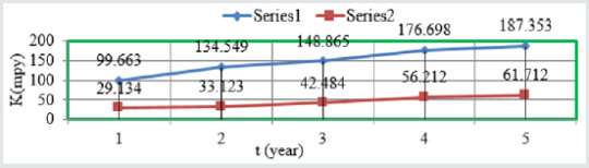
Figure 2: K Vs T for snails at different tempertaures.

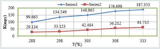
Figure 3: K Vs C for snails at concentations.

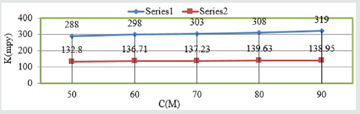
Figure 4: θ Vs T for snails in Aloe Vera.

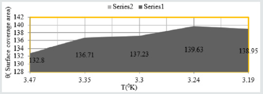
Figure 5: θ Vs C for snails in Aloe Vera.

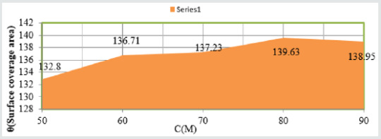
Table 1: Corrosion rate of snail absence and presence of Aloe Vera in H2CO3.

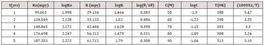
Table 2: Surface coverage area develop by Aloe Vera on the snails in H2CO3.

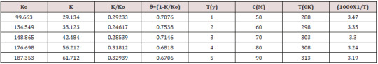
The percentage inhibitors of Aloe Vera at different temperatures and concentrations as one-year interval were calculated by %IE= (1-K/Ko) X100 (where Ko corrosion rate without inhibitor and K corrosion rate with inhibitor) and the values were written in Table 3. The results of Table 3 were depicted that percentage inhibitors efficiency were increased as temperatures and concentration were enhanced. Such types of trends also observed in Figure 6 %IE Vs T and Figure 7 %IE Vs C. Surface adsorption phenomenon was studied by activation energy, heat of adsorption, free energy, enthalpy and entropy. Activation energy was determined by formula K=A e-Ea/RT (where K is corrosion rate, Ea is activation energy and T is absolute temperature without and with action of Aloe Vera at different temperatures and concentrations and their values were recorded in Table 4. It observed that activation energy increased without inhibitors but its values decreased after addition of inhibitors. These results were shown in Table 4 which indicated that inhibitors adhered on snails by chemical bonding and their values were obtained by Figure 8 plotted logK Vs 1/T. Heat of adsorption values were found to be negative which indicated that Aloe Vera was shown an exothermic reaction in H2CO3 medium. It adsorbed on the surface of snail by chemical bonding. The values of heat of adsorption were determined by Langmuir isotherm log(θ/1-θ) = logA +logC-q/2.303RT and Figure 9 plotted log(θ/1-θ) Vs1/T and Figure10 plotted against log(θ/1-θ) Vs logC and their values were recorded in Table 4.

Figure 6: %IE Vs T for snails in Aloe Vera.

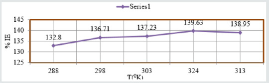
Figure 7: %IE Vs C for snails in Aloe Vera.

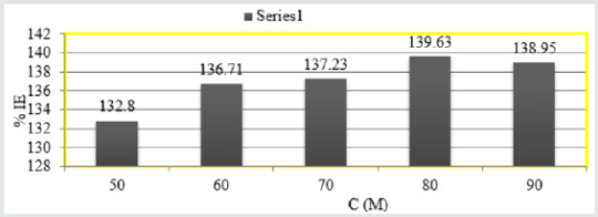
Figure 8: logK Vs 1/T for snails in Aloe Vera.

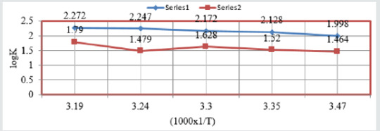
Figure 9: log(θ/1-θ) Vs 1/T for snails in Aloe Vera.

Figure 10: log(θ/1-θ) Vs logC for snails in Aloe Vera.

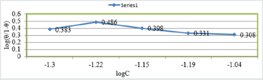
Table 3: Inhibition efficiency develop by Aloe Vera in H2CO3.

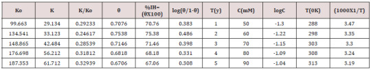
Table 4: Thermal parameters of Aloe Vera with Snails.

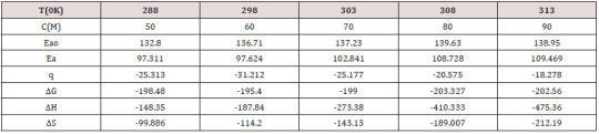
Table 5: Potentiostatic results of snails for Aloe Vera.

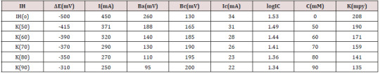
Free energy of inhibitor Aloe Vera was calculated by equation ΔG=2.303 log(33.3K) and their values were given in Table 4. Their values noticed that inhibitor action a chemical reaction because free energy values were negative, and their values mentioned in Table 4. Enthalpy of used inhibitors was determined by transition state equation K=RT/Nh eΔS/R e-ΔH/RT and its values were recorded in Table 4. These values indicated that inhibitor’s Aloe Vera boned with snail by chemical bonding. Entropy of Aloe Vera was determined by equation by ΔG = ΔH – TΔS and their values were mentioned in Table 4. Their values were shown that deposition of Aloe Vera on the surface of snail was an exothermic process. It formed stable barrier on the surface of snail. All five values of thermal parameters plotted against T in Figure 11 and Figure 12 against C. The corrosion potential, corrosion current density and corrosion rate were determined by the equation ΔE/I=1/2.303 βaβc/(βa+βc) and C R(mpy)=0.1288 Ic (mA/cm2) XE/ρ and values were recorded in Table 5. It observed that without inhibitor corrosion potential and corrosion current were decreased but after addition of Aloe Vera corrosion current densities were increased. It also reduced the corrosion potential and corrosion current. The corrosion rate calculated by potentiostat technique and their values were tallied with the corrosion rate determined by gravimetric method. Corrosion potential versus corrosion current density was plotted in Figure 13. This plot indicated that anodic current reduced as addition of inhibitor but cathodic current enhanced Table 5.

Figure 11: Themal energies Vs T for Aloe Vera with Snails.

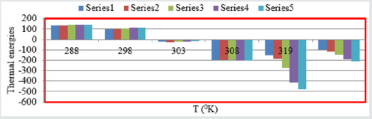
Figure 12: Thermal energies Vs C for Aloe Vera with snails.

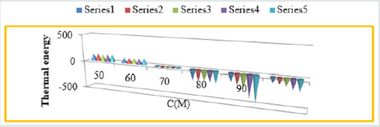
Figure 13: ΔE Vs Ic for snails with Aloe Vera.

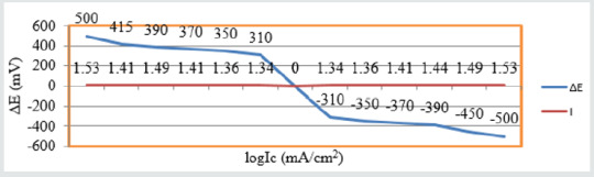
Conclusion

Snails’ corrosion occurs due to change the pH of water. Water pH is altered by contamination effluents, industrial polluters, and various types of wastes and acids rain. Snails outer layers are constructed by calcium carbonate. In acidic medium calcification starts on their surface by chemical process. It produces pitting, stress and crevice corrosion. For the protection of such types corrosion Aloe Vera is used as inhibitors. Aloe Vera forms thin film on the surface of snails. The thin film formation is confirmed by thermal parameters like activation energy, heat of adsorption, free energy, enthalpy and entropy. Aloe Vera surface adsorption phenomenon on snails is also satisfied by Langmuir isotherm. Aloe Vera is reduced the concentration of H+ ions and enhance the concentration of oxygen molecules. It is nitrogen containing rich organic compounds which capture H+ ions and less H2 gas is released thus corroding effect of snails suppressed.

Acknowledgment

Author is thankful for UGC-New Delhi, India for providing financial support for this work. I also thank my research team for their collection of data and graph plotting. I am very grateful professor G Udhayabhanu IITD and professor Sanjoy Misra providing laboratory facility.

For more Lupine Publishers Open Access Journals Please visit our website:

https://lupinepublishers.us/

For more Journal of Modern Approaches on Material Science articles Please Click Here:

https://lupinepublishers.com/material-science-journal/

To Know More About Open Access Publishers Click on Lupine Publishers: https://lupinepublishers.com/

Follow on Linkedin : https://www.linkedin.com/company/lupinepublishers Follow on Twitter : https://twitter.com/lupine_online

#Lupine Publishers #Open Access Journals #Lupine Publishers Group #Material Science Journals #Polymer #composites #biomaterials journal #Biocomposites #Biomedical Engineering #Ceramics

0 notes