#NewClue
Text
KMeans Clustering Assignment
Import the modules
from pandas import Series, DataFrame
import pandas as pd
import numpy as np
import matplotlib.pylab as plt
from sklearn.model_selection import train_test_split
from sklearn import preprocessing
from sklearn.cluster import KMeans
Load the dataset
data = pd.read_csv("C:\Users\guy3404\OneDrive - MDLZ\Documents\Cross Functional Learning\AI COP\Coursera\machine_learning_data_analysis\Datasets\tree_addhealth.csv")
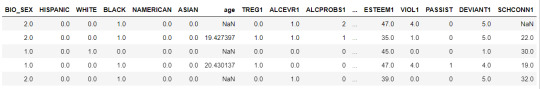
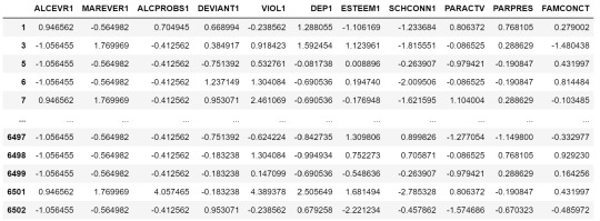
data.head()
upper-case all DataFrame column names
data.columns = map(str.upper, data.columns)
Data Management
data_clean = data.dropna()
data_clean.head()
subset clustering variables
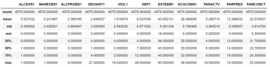
cluster=data_clean[['ALCEVR1','MAREVER1','ALCPROBS1','DEVIANT1','VIOL1',
'DEP1','ESTEEM1','SCHCONN1','PARACTV', 'PARPRES','FAMCONCT']]
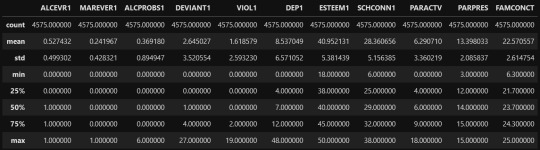
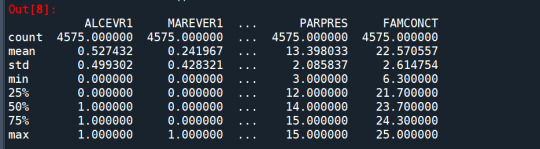
cluster.describe()

standardize clustering variables to have mean=0 and sd=1
clustervar=cluster.copy()
clustervar['ALCEVR1']=preprocessing.scale(clustervar['ALCEVR1'].astype('float64'))
clustervar['ALCPROBS1']=preprocessing.scale(clustervar['ALCPROBS1'].astype('float64'))
clustervar['MAREVER1']=preprocessing.scale(clustervar['MAREVER1'].astype('float64'))
clustervar['DEP1']=preprocessing.scale(clustervar['DEP1'].astype('float64'))
clustervar['ESTEEM1']=preprocessing.scale(clustervar['ESTEEM1'].astype('float64'))
clustervar['VIOL1']=preprocessing.scale(clustervar['VIOL1'].astype('float64'))
clustervar['DEVIANT1']=preprocessing.scale(clustervar['DEVIANT1'].astype('float64'))
clustervar['FAMCONCT']=preprocessing.scale(clustervar['FAMCONCT'].astype('float64'))
clustervar['SCHCONN1']=preprocessing.scale(clustervar['SCHCONN1'].astype('float64'))
clustervar['PARACTV']=preprocessing.scale(clustervar['PARACTV'].astype('float64'))
clustervar['PARPRES']=preprocessing.scale(clustervar['PARPRES'].astype('float64'))
split data into train and test sets
clus_train, clus_test = train_test_split(clustervar, test_size=.3, random_state=123)
k-means cluster analysis for 1-9 clusters
from scipy.spatial.distance import cdist
clusters=range(1,10)
meandist=[]
for k in clusters:
model=KMeans(n_clusters=k)
model.fit(clus_train)
clusassign=model.predict(clus_train)
meandist.append(sum(np.min(cdist(clus_train, model.cluster_centers_, 'euclidean'), axis=1))
/ clus_train.shape[0])
"""
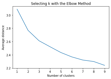
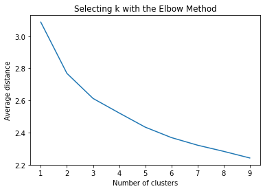
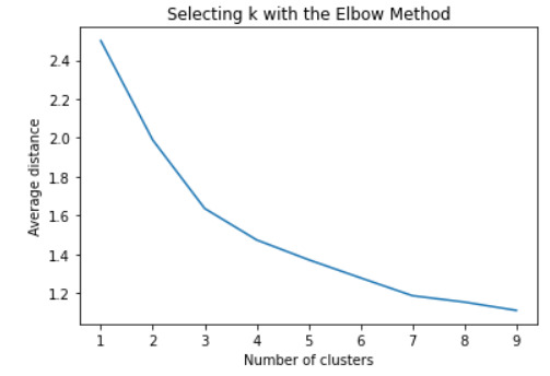
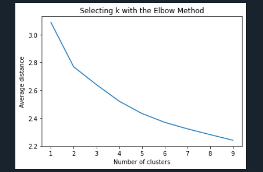
Plot average distance from observations from the cluster centroid
to use the Elbow Method to identify number of clusters to choose
"""
plt.plot(clusters, meandist)
plt.xlabel('Number of clusters')
plt.ylabel('Average distance')
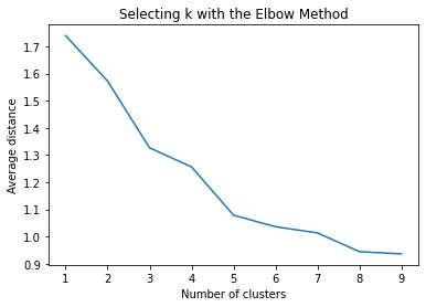
plt.title('Selecting k with the Elbow Method')
Interpret 3 cluster solution
model3=KMeans(n_clusters=3)
model3.fit(clus_train)
clusassign=model3.predict(clus_train)
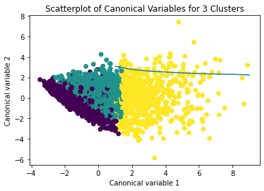
plot clusters
from sklearn.decomposition import PCA
pca_2 = PCA(2)
plot_columns = pca_2.fit_transform(clus_train)
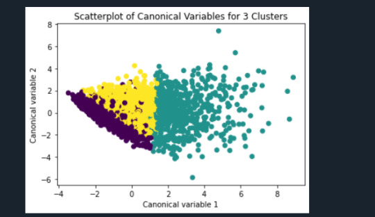
plt.scatter(x=plot_columns[:,0], y=plot_columns[:,1], c=model3.labels_,)
plt.xlabel('Canonical variable 1')
plt.ylabel('Canonical variable 2')
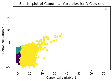
plt.title('Scatterplot of Canonical Variables for 3 Clusters')
plt.show()
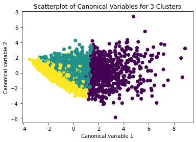
The datapoints of the 2 clusters in the left are less spread out but have more overlaps. The cluster to the right is more distinct but has more spread in the data points
"""
BEGIN multiple steps to merge cluster assignment with clustering variables to examine
cluster variable means by cluster
"""
create a unique identifier variable from the index for the
cluster training data to merge with the cluster assignment variable
clus_train.reset_index(level=0, inplace=True)
create a list that has the new index variable
cluslist=list(clus_train['index'])
create a list of cluster assignments
labels=list(model3.labels_)
combine index variable list with cluster assignment list into a dictionary
newlist=dict(zip(cluslist, labels))
newlist
convert newlist dictionary to a dataframe
newclus=DataFrame.from_dict(newlist, orient='index')
newclus
rename the cluster assignment column
newclus.columns = ['cluster']
now do the same for the cluster assignment variable
create a unique identifier variable from the index for the
cluster assignment dataframe
to merge with cluster training data
newclus.reset_index(level=0, inplace=True)
merge the cluster assignment dataframe with the cluster training variable dataframe
by the index variable
merged_train=pd.merge(clus_train, newclus, on='index')
merged_train.head(n=100)
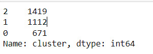
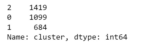
cluster frequencies
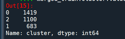
merged_train.cluster.value_counts()
"""
END multiple steps to merge cluster assignment with clustering variables to examine
cluster variable means by cluster
"""
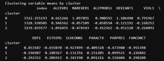
FINALLY calculate clustering variable means by cluster
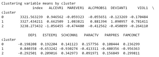
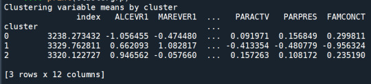
clustergrp = merged_train.groupby('cluster').mean()
print ("Clustering variable means by cluster")
print(clustergrp)
validate clusters in training data by examining cluster differences in GPA using ANOVA
first have to merge GPA with clustering variables and cluster assignment data
gpa_data=data_clean['GPA1']
split GPA data into train and test sets
gpa_train, gpa_test = train_test_split(gpa_data, test_size=.3, random_state=123)
gpa_train1=pd.DataFrame(gpa_train)
gpa_train1.reset_index(level=0, inplace=True)
merged_train_all=pd.merge(gpa_train1, merged_train, on='index')
sub1 = merged_train_all[['GPA1', 'cluster']].dropna()
Print statistical summary by cluster
import statsmodels.formula.api as smf
import statsmodels.stats.multicomp as multi
gpamod = smf.ols(formula='GPA1 ~ C(cluster)', data=sub1).fit()
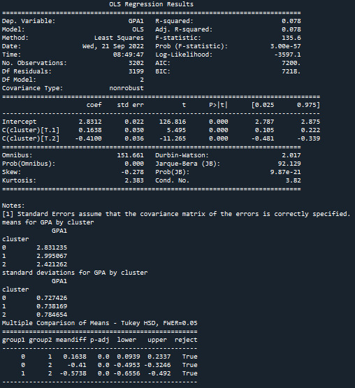
print (gpamod.summary())
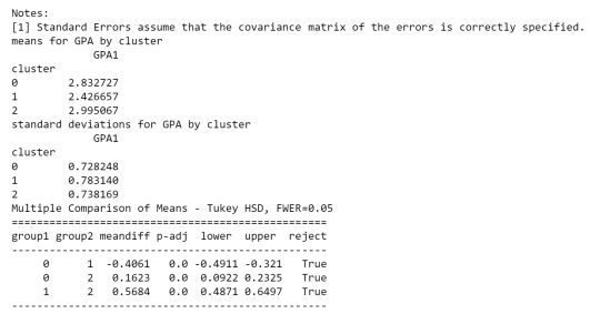
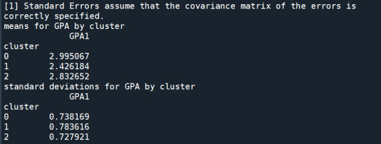
print ('means for GPA by cluster')
m1= sub1.groupby('cluster').mean()
print (m1)
print ('standard deviations for GPA by cluster')
m2= sub1.groupby('cluster').std()
print (m2)
Interpretation
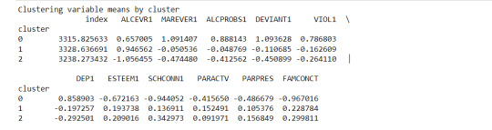
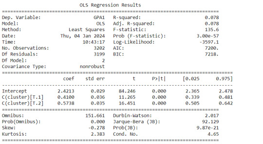
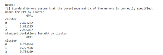
The clustering average summary shows Cluster 0 has higher alcohol and marijuana problems, shows higher deviant and violent behavior, suffers from depression, has low self esteem,school connectedness, paraental and family connectedness. On the contrary, Cluster 2 shows the lowest alcohol and marijuana problems, lowest deviant & violent behavior,depression, and higher self esteem,school connectedness, paraental and family connectedness. Further, when validated against GPA score, we observe Cluster 0 shows the lowest average GPA and CLuster 2 has the highest average GPA which aligns with the summary statistics interpretation.
0 notes
Text
input:
from pandas import Series, DataFrame
import pandas as pd
import numpy as np
import matplotlib.pylab as plt
from sklearn.model_selection import train_test_split
from sklearn import preprocessing
from sklearn.cluster import KMeans
from scipy.spatial.distance import cdist
from sklearn.decomposition import PCA
import statsmodels.formula.api as smf
import statsmodels.stats.multicomp as
multi data = pd.read_csv("./archive/tree_addhealth.csv")
data.columns = map(str.upper, data.columns)
data_clean = data.dropna()
cluster=data_clean[['ALCEVR1','MAREVER1','ALCPROBS1','DEVIANT1','VIOL1','DEP1','ESTEEM1','SCHCONN1','PARACTV', 'PARPRES','FAMCONCT']]
output:
clustervar=cluster.copy()
clustervar['ALCEVR1']=preprocessing.scale(clustervar['ALCEVR1'].astype('float64'))
clustervar['ALCPROBS1']=preprocessing.scale(clustervar['ALCPROBS1'].astype('float64'))
clustervar['MAREVER1']=preprocessing.scale(clustervar['MAREVER1'].astype('float64'))
clustervar['DEP1']=preprocessing.scale(clustervar['DEP1'].astype('float64'))
clustervar['ESTEEM1']=preprocessing.scale(clustervar['ESTEEM1'].astype('float64'))
clustervar['VIOL1']=preprocessing.scale(clustervar['VIOL1'].astype('float64'))
clustervar['DEVIANT1']=preprocessing.scale(clustervar['DEVIANT1'].astype('float64'))
clustervar['FAMCONCT']=preprocessing.scale(clustervar['FAMCONCT'].astype('float64'))
clustervar['SCHCONN1']=preprocessing.scale(clustervar['SCHCONN1'].astype('float64'))
clustervar['PARACTV']=preprocessing.scale(clustervar['PARACTV'].astype('float64'))
clustervar['PARPRES']=preprocessing.scale(clustervar['PARPRES'].astype('float64'))
clus_train, clus_test = train_test_split(clustervar, test_size=.3, random_state=123)
clusters=range(1,10)meandist=[]
for k in clusters:
model=KMeans(n_clusters=k)
model.fit(clus_train)
clusassign=model.predict(clus_train)
meandist.append(sum(np.min(cdist(clus_train, model.cluster_centers_, 'euclidean'), axis=1))
/ clus_train.shape[0])
plt.plot(clusters, meandist)
plt.xlabel('Number of clusters')
plt.ylabel('Average distance')
plt.title('Selecting k with the Elbow Method')
output:
model3=KMeans(n_clusters=3)
model3.fit(clus_train)
clusassign=model3.predict(clus_train)
pca_2 = PCA(2)
plot_columns = pca_2.fit_transform(clus_train)
plt.scatter(x=plot_columns[:,0], y=plot_columns[:,1], c=model3.labels_,)
plt.xlabel('Canonical variable 1')
plt.ylabel('Canonical variable 2')
plt.title('Scatterplot of Canonical Variables for 3 Clusters')
plt.show()
output:

clus_train.reset_index(level=0, inplace=True)
cluslist=list(clus_train['index'])
labels=list(model3.labels_)
newlist=dict(zip(cluslist, labels))
newlist
newclus=DataFrame.from_dict(newlist, orient='index')
newclus
newclus.columns = ['cluster']
newclus.reset_index(level=0, inplace=True)
merged_train=pd.merge(clus_train, newclus, on='index')
merged_train.head(n=100)
merged_train.cluster.value_counts()
output:
2 1420
1 1108
0 674
Name: cluster, dtype: int64
clustergrp = merged_train.groupby('cluster').mean()
print ("Clustering variable means by cluster")
print(clustergrp)
output:
gpa_data=data_clean['GPA1']
gpa_train, gpa_test = train_test_split(gpa_data, test_size=.3, random_state=123)
gpa_train1=pd.DataFrame(gpa_train)
gpa_train1.reset_index(level=0, inplace=True)
merged_train_all=pd.merge(gpa_train1, merged_train, on='index')
sub1 = merged_train_all[['GPA1', 'cluster']].dropna()
gpamod = smf.ols(formula='GPA1 ~ C(cluster)', data=sub1).fit()
print (gpamod.summary())
print ('means for GPA by cluster')
m1= sub1.groupby('cluster').mean()
print (m1)
print ('standard deviations for GPA by cluster')
m2= sub1.groupby('cluster').std()
print (m2)
mc1 = multi.MultiComparison(sub1['GPA1'], sub1['cluster'])
res1 = mc1.tukeyhsd()
print(res1.summary())
ouput:

0 notes
Text
rom pandas import Series, DataFrame
import pandas as pd
import numpy as np
import matplotlib.pylab as plt
from sklearn.model_selection import train_test_split
from sklearn import preprocessing
from sklearn.cluster import KMeans
"""
Data Management
"""
data = pd.read_csv("tree_addhealth")
upper-case all DataFrame column names
data.columns = map(str.upper, data.columns)
Data Management
data_clean = data.dropna()
subset clustering variables
cluster=data_clean[['ALCEVR1','MAREVER1','ALCPROBS1','DEVIANT1','VIOL1',
'DEP1','ESTEEM1','SCHCONN1','PARACTV', 'PARPRES','FAMCONCT']]
cluster.describe()
standardize clustering variables to have mean=0 and sd=1
clustervar=cluster.copy()
clustervar['ALCEVR1']=preprocessing.scale(clustervar['ALCEVR1'].astype('float64'))
clustervar['ALCPROBS1']=preprocessing.scale(clustervar['ALCPROBS1'].astype('float64'))
clustervar['MAREVER1']=preprocessing.scale(clustervar['MAREVER1'].astype('float64'))
clustervar['DEP1']=preprocessing.scale(clustervar['DEP1'].astype('float64'))
clustervar['ESTEEM1']=preprocessing.scale(clustervar['ESTEEM1'].astype('float64'))
clustervar['VIOL1']=preprocessing.scale(clustervar['VIOL1'].astype('float64'))
clustervar['DEVIANT1']=preprocessing.scale(clustervar['DEVIANT1'].astype('float64'))
clustervar['FAMCONCT']=preprocessing.scale(clustervar['FAMCONCT'].astype('float64'))
clustervar['SCHCONN1']=preprocessing.scale(clustervar['SCHCONN1'].astype('float64'))
clustervar['PARACTV']=preprocessing.scale(clustervar['PARACTV'].astype('float64'))
clustervar['PARPRES']=preprocessing.scale(clustervar['PARPRES'].astype('float64'))
split data into train and test sets
clus_train, clus_test = train_test_split(clustervar, test_size=.3, random_state=123)
k-means cluster analysis for 1-9 clusters
from scipy.spatial.distance import cdist
clusters=range(1,10)
meandist=[]
for k in clusters:
model=KMeans(n_clusters=k)
model.fit(clus_train)
clusassign=model.predict(clus_train)
meandist.append(sum(np.min(cdist(clus_train, model.cluster_centers_, 'euclidean'), axis=1))
/ clus_train.shape[0])
"""
Plot average distance from observations from the cluster centroid
to use the Elbow Method to identify number of clusters to choose
"""
plt.plot(clusters, meandist)
plt.xlabel('Number of clusters')
plt.ylabel('Average distance')
plt.title('Selecting k with the Elbow Method')
Interpret 3 cluster solution
model3=KMeans(n_clusters=3)
model3.fit(clus_train)
clusassign=model3.predict(clus_train)
plot clusters
from sklearn.decomposition import PCA
pca_2 = PCA(2)
plot_columns = pca_2.fit_transform(clus_train)
plt.scatter(x=plot_columns[:,0], y=plot_columns[:,1], c=model3.labels_,)
plt.xlabel('Canonical variable 1')
plt.ylabel('Canonical variable 2')
plt.title('Scatterplot of Canonical Variables for 3 Clusters')
plt.show()
"""
BEGIN multiple steps to merge cluster assignment with clustering variables to examine
cluster variable means by cluster
"""
create a unique identifier variable from the index for the
cluster training data to merge with the cluster assignment variable
clus_train.reset_index(level=0, inplace=True)
create a list that has the new index variable
cluslist=list(clus_train['index'])
create a list of cluster assignments
labels=list(model3.labels_)
combine index variable list with cluster assignment list into a dictionary
newlist=dict(zip(cluslist, labels))
newlist
convert newlist dictionary to a dataframe
newclus=DataFrame.from_dict(newlist, orient='index')
newclus
rename the cluster assignment column
newclus.columns = ['cluster']
now do the same for the cluster assignment variable
create a unique identifier variable from the index for the
cluster assignment dataframe
to merge with cluster training data
newclus.reset_index(level=0, inplace=True)
merge the cluster assignment dataframe with the cluster training variable dataframe
by the index variable
merged_train=pd.merge(clus_train, newclus, on='index')
merged_train.head(n=100)
cluster frequencies
merged_train.cluster.value_counts()
"""
END multiple steps to merge cluster assignment with clustering variables to examine
cluster variable means by cluster
"""
FINALLY calculate clustering variable means by cluster
clustergrp = merged_train.groupby('cluster').mean()
print ("Clustering variable means by cluster")
print(clustergrp)
validate clusters in training data by examining cluster differences in GPA using ANOVA
first have to merge GPA with clustering variables and cluster assignment data
gpa_data=data_clean['GPA1']
split GPA data into train and test sets
gpa_train, gpa_test = train_test_split(gpa_data, test_size=.3, random_state=123)
gpa_train1=pd.DataFrame(gpa_train)
gpa_train1.reset_index(level=0, inplace=True)
merged_train_all=pd.merge(gpa_train1, merged_train, on='index')
sub1 = merged_train_all[['GPA1', 'cluster']].dropna()
import statsmodels.formula.api as smf
import statsmodels.stats.multicomp as multi
gpamod = smf.ols(formula='GPA1 ~ C(cluster)', data=sub1).fit()
print (gpamod.summary())
print ('means for GPA by cluster')
m1= sub1.groupby('cluster').mean()
print (m1)
print ('standard deviations for GPA by cluster')
m2= sub1.groupby('cluster').std()
print (m2)
mc1 = multi.MultiComparison(sub1['GPA1'], sub1['cluster'])
res1 = mc1.tukeyhsd()
print(res1.summary())
0 notes
Text
Machine Learning for Data Analysis - Week 4
#Load the data and convert the variables to numeric
import pandas as pd
import numpy as np
import matplotlib.pyplot as plt
from sklearn.model_selection import train_test_split
from sklearn.linear_model import LassoLarsCV
import statsmodels.formula.api as smf
import statsmodels.stats.multicomp as multi
from sklearn import preprocessing
from sklearn.cluster import KMeans
data = pd.read_csv('gapminder.csv', low_memory=False)
data['urbanrate'] = pd.to_numeric(data['urbanrate'], errors='coerce')
data['incomeperperson'] = pd.to_numeric(data['incomeperperson'], errors='coerce')
data['femaleemployrate'] = pd.to_numeric(data['femaleemployrate'], errors='coerce')
data['breastcancerper100th'] = pd.to_numeric(data['breastcancerper100th'], errors='coerce')
data['internetuserate'] = pd.to_numeric(data['internetuserate'], errors='coerce')
data['employrate'] = pd.to_numeric(data['employrate'], errors='coerce')
data['polityscore'] = pd.to_numeric(data['polityscore'], errors='coerce')
data['lifeexpectancy'] = pd.to_numeric(data['lifeexpectancy'], errors='coerce')
sub1 = data.copy()
data_clean = sub1.dropna()
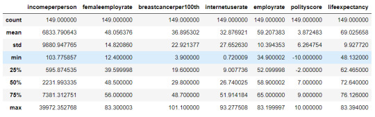
#Subset the clustering variables
cluster = data_clean[['incomeperperson','femaleemployrate','breastcancerper100th','internetuserate',
'employrate', 'polityscore', 'lifeexpectancy']]
cluster.describe()
#Standardize the clustering variables to have mean = 0 and standard deviation = 1
clustervar=cluster.copy()
clustervar['incomeperperson']=preprocessing.scale(clustervar['incomeperperson'].astype('float64'))
clustervar['femaleemployrate']=preprocessing.scale(clustervar['femaleemployrate'].astype('float64'))
clustervar['breastcancerper100th']=preprocessing.scale(clustervar['breastcancerper100th'].astype('float64'))
clustervar['internetuserate']=preprocessing.scale(clustervar['internetuserate'].astype('float64'))
clustervar['employrate']=preprocessing.scale(clustervar['employrate'].astype('float64'))
clustervar['polityscore']=preprocessing.scale(clustervar['polityscore'].astype('float64'))
clustervar['lifeexpectancy']=preprocessing.scale(clustervar['lifeexpectancy'].astype('float64'))
#Split the data into train and test sets
clus_train, clus_test = train_test_split(clustervar, test_size=.3, random_state=123)
#Perform k-means cluster analysis for 1-9 clusters
from scipy.spatial.distance import cdist
clusters = range(1,10)
meandist = []
for k in clusters:
model = KMeans(n_clusassign = k)
model.fit(clus_train)
clusters = model.predict(clus_train)
meandist.append(sum(np.min(cdist(clus_train, model.cluster_centers_, 'euclidean'), axis=1))
/ clus_train.shape[0])
#Plot average distance from observations from the cluster centroid to use the Elbow Method to identify number of clusters to choose
plt.plot(clusters, meandist)
plt.xlabel('Number of clusters')
plt.ylabel('Average distance')
plt.title('Selecting k with the Elbow Method')
plt.show()
#Interpret 3 cluster solution
model3 = KMeans(n_clusters=4)
model3.fit(clus_train)
clusassign = model3.predict(clus_train)
#Plot the clusters
from sklearn.decomposition import PCA
pca_2 = PCA(2)
plt.figure()
plot_columns = pca_2.fit_transform(clus_train)
plt.scatter(x=plot_columns[:,0], y=plot_columns[:,1], c=model3.labels_,)
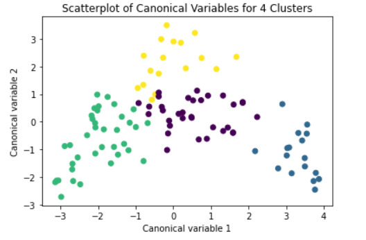
plt.xlabel('Canonical variable 1')
plt.ylabel('Canonical variable 2')
plt.title('Scatterplot of Canonical Variables for 4 Clusters')
plt.show()
#Create a unique identifier variable from the index for the cluster training data to merge with the cluster assignment variable.
clus_train.reset_index(level=0, inplace=True)
#Create a list that has the new index variable
cluslist = list(clus_train['index'])
#Create a list of cluster assignments
labels = list(model3.labels_)
#Combine index variable list with cluster assignment list into a dictionary
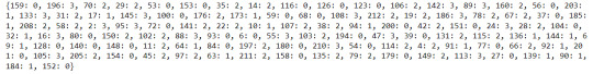
newlist = dict(zip(cluslist, labels))
print(newlist)
#Convert newlist dictionary to a dataframe
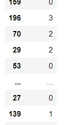
newclus = pd.DataFrame.from_dict(newlist, orient='index')
#Rename the cluster assignment column
newclus.columns = ['cluster']
newclus
#Create a unique identifier variable from the index for the cluster assignment dataframe to merge with cluster training data
newclus.reset_index(level=0, inplace=True)
#Merge the cluster assignment dataframe with the cluster training variable dataframe by the index variable
merged_train = pd.merge(clus_train, newclus, on='index')
merged_train.head(n=100)
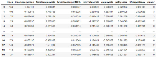
#Cluster frequencies
merged_train.cluster.value_counts()

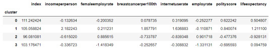
#Calculate clustering variable means by cluster
clustergrp = merged_train.groupby('cluster').mean()
print ("Clustering variable means by cluster")
clustergrp
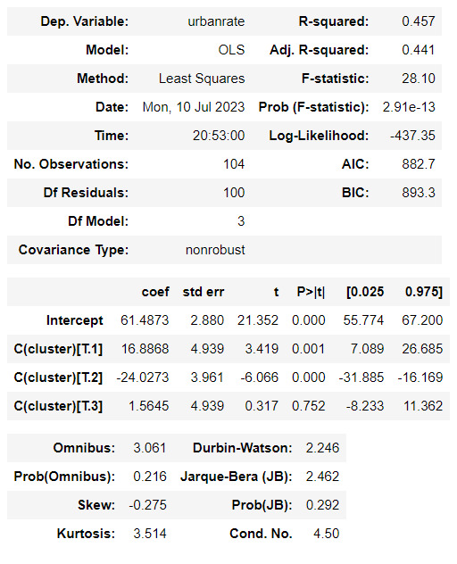
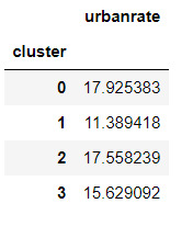
#Validate clusters in training data by examining cluster differences in urbanrate using ANOVA.
#First, merge urbanrate with clustering variables and cluster assignment data
urbanrate_data = data_clean['urbanrate']
#Split urbanrate data into train and test sets
urbanrate_train, internetuserate_test = train_test_split(urbanrate_data, test_size=.3, random_state=123)
urbanrate_train1=pd.DataFrame(urbanrate_train)
urbanrate_train1.reset_index(level=0, inplace=True)
merged_train_all=pd.merge(urbanrate_train1, merged_train, on='index')
sub5 = merged_train_all[['urbanrate', 'cluster']].dropna()
urbanrate_mod = smf.ols(formula='urbanrate ~ C(cluster)', data=sub5).fit()
urbanrate_mod.summary()
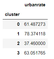
#Means for urbanrate by cluster
m1= sub5.groupby('cluster').mean()
m1
#Standard deviations for urbanrate by cluster
m2= sub5.groupby('cluster').std()
m2
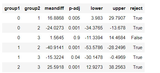
mc1 = multi.MultiComparison(sub5['urbanrate'], sub5['cluster'])
res1 = mc1.tukeyhsd()
res1.summary()
0 notes
Text
Código K- means craters of mars
-- coding: utf-8 --
"""
Created on Fri Jun 16 19:08:39 2023
@author: ANGELA
"""
from pandas import Series, DataFrame
import pandas
import numpy as np
import matplotlib.pylab as plt
from sklearn.model_selection import train_test_split
from sklearn import preprocessing
from sklearn.cluster import KMeans
"""Data management"""
data = pandas.read_csv('marscrater_pds.csv', low_memory=False)
data['LATITUDE_CIRCLE_IMAGE']=pandas.to_numeric(data['LATITUDE_CIRCLE_IMAGE'],errors='coerce')
data['LONGITUDE_CIRCLE_IMAGE']=pandas.to_numeric(data['LONGITUDE_CIRCLE_IMAGE'],errors='coerce')
data['DIAM_CIRCLE_IMAGE']=pandas.to_numeric(data['DIAM_CIRCLE_IMAGE'],errors='coerce')
data['NUMBER_LAYERS']=pandas.to_numeric(data['NUMBER_LAYERS'],errors='coerce')
data['DEPTH_RIMFLOOR_TOPOG']=pandas.to_numeric(data['DEPTH_RIMFLOOR_TOPOG'],errors='coerce')
upper-case all DataFrame column names
data.columns = map(str.upper, data.columns)
data_clean =data.dropna()
target = data_clean.DEPTH_RIMFLOOR_TOPOG
select predictor variables and target variable as separate data sets
cluster= data_clean[['LATITUDE_CIRCLE_IMAGE','LONGITUDE_CIRCLE_IMAGE','DIAM_CIRCLE_IMAGE']]
cluster.describe()
standardize clustering variables to have mean=0 and sd=1
clustervar=cluster.copy()
clustervar['LATITUDE_CIRCLE_IMAGE']=preprocessing.scale(clustervar['LATITUDE_CIRCLE_IMAGE'].astype('float64'))
clustervar['LONGITUDE_CIRCLE_IMAGE']=preprocessing.scale(clustervar['LONGITUDE_CIRCLE_IMAGE'].astype('float64'))
clustervar['DIAM_CIRCLE_IMAGE']=preprocessing.scale(clustervar['DIAM_CIRCLE_IMAGE'].astype('float64'))
clustervar['DEPTH_RIMFLOOR_TOPOG']=preprocessing.scale(clustervar['DEPTH_RIMFLOOR_TOPOG'].astype('float64'))
split data into train and test sets
clus_train, clus_test = train_test_split(clustervar, test_size=.3, random_state=200)
k-means cluster analysis for 1-9 clusters
from scipy.spatial.distance import cdist
clusters=range(1,10)
meandist=[]
Calculate cluster
for k in clusters:
model=KMeans(n_clusters=k)
model.fit(clus_train)
clusassign=model.predict(clus_train)
meandist.append(sum(np.min(cdist(clus_train, model.cluster_centers_, 'euclidean'), axis=1))
/ clus_train.shape[0])
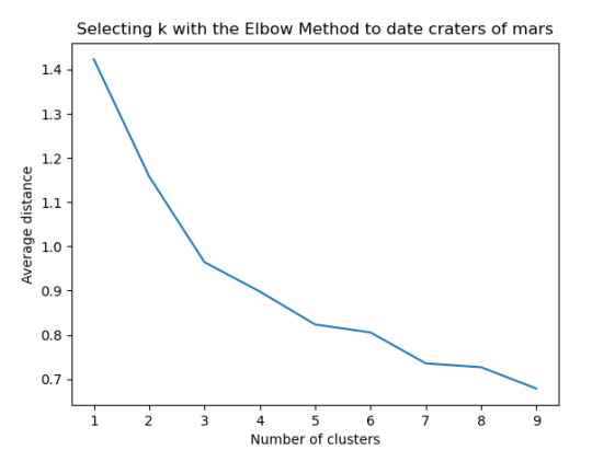
"""
Plot average distance from observations from the cluster centroid
to use the Elbow Method to identify number of clusters to choose
"""
plt.plot(clusters, meandist)
plt.xlabel('Number of clusters')
plt.ylabel('Average distance')
plt.title('Selecting k with the Elbow Method to date craters of mars')
Interpret 3 cluster solution
model3=KMeans(n_clusters=3)
model3.fit(clus_train)
clusassign=model3.predict(clus_train)
plot clusters
from sklearn.decomposition import PCA
pca_2 = PCA(2)
plot_columns = pca_2.fit_transform(clus_train)
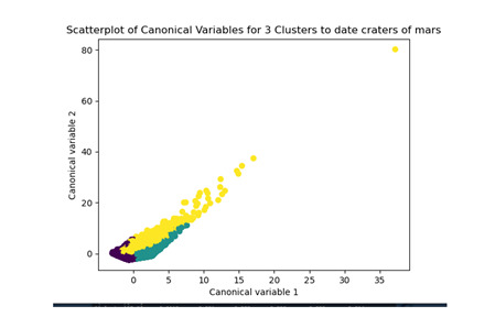
plt.scatter(x=plot_columns[:,0], y=plot_columns[:,1], c=model3.labels_,)
plt.xlabel('Canonical variable 1')
plt.ylabel('Canonical variable 2')
plt.title('Scatterplot of Canonical Variables for 3 Clusters to date craters of mars')
plt.show()
"""
BEGIN multiple steps to merge cluster assignment with clustering variables to examine
cluster variable means by cluster
"""
create a unique identifier variable from the index for the
cluster training data to merge with the cluster assignment variable
clus_train.reset_index(level=0, inplace=True)
create a list that has the new index variable
cluslist=list(clus_train['index'])
create a list of cluster assignments
labels=list(model3.labels_)
combine index variable list with cluster assignment list into a dictionary
newlist=dict(zip(cluslist, labels))
newlist
convert newlist dictionary to a dataframe
newclus=DataFrame.from_dict(newlist, orient='index')
newclus
rename the cluster assignment column
newclus.columns = ['cluster']
now do the same for the cluster assignment variable
create a unique identifier variable from the index for the
cluster assignment dataframe
to merge with cluster training data
newclus.reset_index(level=0, inplace=True)
merge the cluster assignment dataframe with the cluster training variable dataframe
by the index variable
merged_train=pandas.merge(clus_train, newclus, on='index')
merged_train.head(n=100)
cluster frequencies
merged_train.cluster.value_counts()
"""
END multiple steps to merge cluster assignment with clustering variables to examine
cluster variable means by cluster
"""
FINALLY calculate clustering variable means by cluster
clustergrp = merged_train.groupby('cluster').mean()
print ("Clustering variable means by cluster")
print(clustergrp)
validate clusters in training data by examining cluster differences in DEPTH_RIMFLOOR_TOPOG using ANOVA
first have to merge DEPTH_RIMFLOOR_TOPOG with clustering variables and cluster assignment data
DRT_data=data_clean['DEPTH_RIMFLOOR_TOPOG']
split DEPTH_RIMFLOOR_TOPOG data into train and test sets
DRT_train, DRT_test = train_test_split(DRT_data, test_size=.3, random_state=123)
DRT_train1=pandas.DataFrame(DRT_train)
DRT_train1.reset_index(level=0, inplace=True)
merged_train_all=pandas.merge(DRT_train1, merged_train, on='index')
sub1 = merged_train_all[['DEPTH_RIMFLOOR_TOPOG', 'cluster']].dropna()
import statsmodels.formula.api as smf
import statsmodels.stats.multicomp as multi
DTRmod = smf.ols(formula='DEPTH_RIMFLOOR_TOPOG ~ C(cluster)', data=sub1).fit()
print (DTRmod.summary())
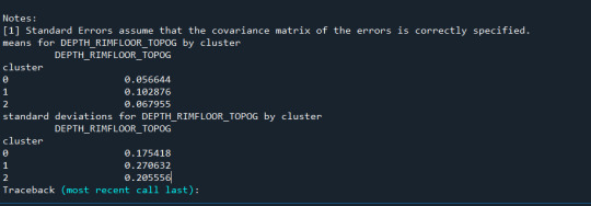
print ('means for DEPTH_RIMFLOOR_TOPOG by cluster')
m1= sub1.groupby('cluster').mean()
print (m1)
print ('standard deviations for DEPTH_RIMFLOOR_TOPOG by cluster')
m2= sub1.groupby('cluster').std()
print (m2)
mc1 = multi.MultiComparison(sub1['GPA1'], sub1['cluster'])
res1 = mc1.tukeyhsd()
print(res1.summary())
Resultados
Los cluster posibles son 3, 5, 7 y 8 donde se evidencia un punto de quiebre en la ilustración, por lo que se realizó la prueba con 3 clusters y se evidencia que puede presentarse un overfiting al esta muy cerca y cobre puestos los clusters

0 notes
Text
MOD 4
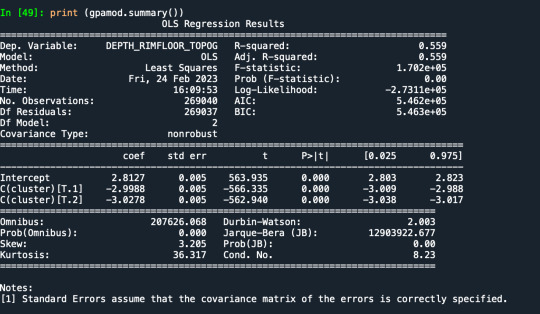
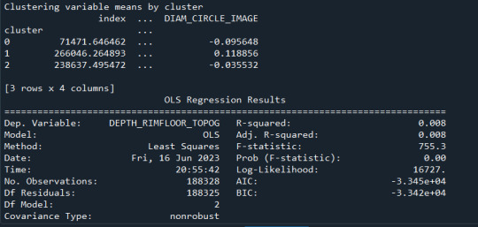
Results from the OLS regression results using the depth rim floor as the variable. the numbers appear to be close and now too far off. Cluster 0 having the biggest depth rim floor to the top.
demonstrates that there is a giant overlap within the cluster groups however the yellow group appears to be more dispersed.
shows that theyre may be overlaps values 2, 3, 4, 5,6,7,8. This means that the variables being utilized are similar. Therefore the canonical variable test was performed to reduce the number of available variables.
CODE SCRIPT
from pandas import Series, DataFrame
import pandas as pd
import numpy as np
import matplotlib.pylab as plt
from sklearn.model_selection import train_test_split
from sklearn import preprocessing
from sklearn.cluster import KMeans
"""
Data Management
"""
data = pd.read_csv('https://d3c33hcgiwev3.cloudfront.net/2c7ec69d0edd3b9599c0df80f0901a52_marscrater_pds.csv?Expires=1677369600&Signature=YDtfrRGhpLU3YbElRnuT3BynxPQdU1s3n6D-tR~Kb1tv7gDGdw2cKF49yGsmou3zWhP4ScXqbCGPbSdTd8SCPdZQpGXuj5B9I2lpUXObnn3OWFsNlQDz7WmrsngPFSdWHciEYCpCdYegyMmghimmDw1xZepgByZPuB5-Z6b3fOQ&Key-Pair-Id=APKAJLTNE6QMUY6HBC5A')
upper-case all DataFrame column names
data.columns = map(str.upper, data.columns)
Data Management
data_clean = data.dropna()
data.dtypes
subset clustering variables
cluster=data_clean[['LATITUDE_CIRCLE_IMAGE','LONGITUDE_CIRCLE_IMAGE','DIAM_CIRCLE_IMAGE','DEPTH_RIMFLOOR_TOPOG',
'NUMBER_LAYERS']]
cluster.describe()
standardize clustering variables to have mean=0 and sd=1
clustervar=cluster.copy()
clustervar['LATITUDE_CIRCLE_IMAGE']=preprocessing.scale(clustervar['LATITUDE_CIRCLE_IMAGE'].astype('float64'))
clustervar['LONGITUDE_CIRCLE_IMAGE']=preprocessing.scale(clustervar['LONGITUDE_CIRCLE_IMAGE'].astype('float64'))
clustervar['DIAM_CIRCLE_IMAGE']=preprocessing.scale(clustervar['DIAM_CIRCLE_IMAGE'].astype('float64'))
clustervar['DEPTH_RIMFLOOR_TOPOG']=preprocessing.scale(clustervar['DEPTH_RIMFLOOR_TOPOG'].astype('float64'))
clustervar['NUMBER_LAYERS']=preprocessing.scale(clustervar['NUMBER_LAYERS'].astype('float64'))
split data into train and test sets
clus_train, clus_test = train_test_split(clustervar, test_size=.3, random_state=123)
k-means cluster analysis for 1-9 clusters
from scipy.spatial.distance import cdist
clusters=range(1,10)
meandist=[]
for k in clusters:
model=KMeans(n_clusters=k)
model.fit(clus_train)
clusassign=model.predict(clus_train)
meandist.append(sum(np.min(cdist(clus_train, model.cluster_centers_, 'euclidean'), axis=1))
/ clus_train.shape[0])
"""
Plot average distance from observations from the cluster centroid
to use the Elbow Method to identify number of clusters to choose
"""
plt.plot(clusters, meandist)
plt.xlabel('Number of clusters')
plt.ylabel('Average distance')
plt.title('Selecting k with the Elbow Method')
Interpret 3 cluster solution
model3=KMeans(n_clusters=3)
model3.fit(clus_train)
clusassign=model3.predict(clus_train)
plot clusters
from sklearn.decomposition import PCA
pca_2 = PCA(2)
plot_columns = pca_2.fit_transform(clus_train)
plt.scatter(x=plot_columns[:,0], y=plot_columns[:,1], c=model3.labels_,)
plt.xlabel('Canonical variable 1')
plt.ylabel('Canonical variable 2')
plt.title('Scatterplot of Canonical Variables for 3 Clusters')
plt.show()
"""
BEGIN multiple steps to merge cluster assignment with clustering variables to examine
cluster variable means by cluster
"""
create a unique identifier variable from the index for the
cluster training data to merge with the cluster assignment variable
clus_train.reset_index(level=0, inplace=True)
create a list that has the new index variable
cluslist=list(clus_train['index'])
create a list of cluster assignments
labels=list(model3.labels_)
combine index variable list with cluster assignment list into a dictionary
newlist=dict(zip(cluslist, labels))
newlist
convert newlist dictionary to a dataframe
newclus=DataFrame.from_dict(newlist, orient='index')
newclus
rename the cluster assignment column
newclus.columns = ['cluster']
now do the same for the cluster assignment variable
create a unique identifier variable from the index for the
cluster assignment dataframe
to merge with cluster training data
newclus.reset_index(level=0, inplace=True)
merge the cluster assignment dataframe with the cluster training variable dataframe
by the index variable
merged_train=pd.merge(clus_train, newclus, on='index')
merged_train.head(n=100)
cluster frequencies
merged_train.cluster.value_counts()
"""
END multiple steps to merge cluster assignment with clustering variables to examine
cluster variable means by cluster
"""
FINALLY calculate clustering variable means by cluster
clustergrp = merged_train.groupby('cluster').mean()
print ("Clustering variable means by cluster")
print(clustergrp)
validate clusters in training data by examining cluster differences in GPA using ANOVA
first have to merge GPA with clustering variables and cluster assignment data
depth_data=data_clean['DEPTH_RIMFLOOR_TOPOG']
split GPA data into train and test sets
depth_train, depth_test = train_test_split(depth_data, test_size=.3, random_state=123)
depth_train1=pd.DataFrame(layer_train)
depth_train1.reset_index(level=0, inplace=True)
merged_train_all=pd.merge(depth_train1, merged_train, on='index')
sub1 = merged_train_all[['DEPTH_RIMFLOOR_TOPOG', 'cluster']].dropna()
import statsmodels.formula.api as smf
import statsmodels.stats.multicomp as multi
gpamod = smf.ols(formula='DEPTH_RIMFLOOR_TOPOG ~ C(cluster)', data=sub1).fit()
print (gpamod.summary())
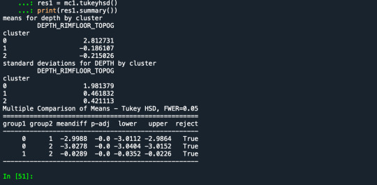
print ('means for depth by cluster')
m1= sub1.groupby('cluster').mean()
print (m1)
print ('standard deviations for DEPTH by cluster')
m2= sub1.groupby('cluster').std()
print (m2)
mc1 = multi.MultiComparison(sub1['DEPTH_RIMFLOOR_TOPOG'], sub1['cluster'])
res1 = mc1.tukeyhsd()
print(res1.summary())
0 notes
Text
K-Means Clustering
1. Data
I used the data "tree_addhealth.csv" for my coursera K-means assignment. This analysis was conducted in Python.
The variables selected to perform the clustering data were:
cluster=data_clean[['ALCEVR1','MAREVER1','ALCPROBS1','DEVIANT1','VIOL1',
'DEP1','ESTEEM1','SCHCONN1','PARACTV', 'PARPRES','FAMCONCT']]
cluster.describe()
2. Code
On the other hand, the code used to perform the analysis is the following:
---- START CODE ----
from pandas import Series, DataFrame
import pandas as pd
import numpy as np
import matplotlib.pylab as plt
from sklearn.model_selection import train_test_split
from sklearn import preprocessing
from sklearn.cluster import KMeans
import os
os.chdir("../data/")
"""
Data Management
"""
data = pd.read_csv("tree_addhealth.csv")
data.columns = map(str.upper, data.columns)
data_clean = data.dropna()
cluster=data_clean[['ALCEVR1','MAREVER1','ALCPROBS1','DEVIANT1','VIOL1',
'DEP1','ESTEEM1','SCHCONN1','PARACTV', 'PARPRES','FAMCONCT']]
cluster.describe()
clustervar=cluster.copy()
clustervar['ALCEVR1']=preprocessing.scale(clustervar['ALCEVR1'].astype('float64'))
clustervar['ALCPROBS1']=preprocessing.scale(clustervar['ALCPROBS1'].astype('float64'))
clustervar['MAREVER1']=preprocessing.scale(clustervar['MAREVER1'].astype('float64'))
clustervar['DEP1']=preprocessing.scale(clustervar['DEP1'].astype('float64'))
clustervar['ESTEEM1']=preprocessing.scale(clustervar['ESTEEM1'].astype('float64'))
clustervar['VIOL1']=preprocessing.scale(clustervar['VIOL1'].astype('float64'))
clustervar['DEVIANT1']=preprocessing.scale(clustervar['DEVIANT1'].astype('float64'))
clustervar['FAMCONCT']=preprocessing.scale(clustervar['FAMCONCT'].astype('float64'))
clustervar['SCHCONN1']=preprocessing.scale(clustervar['SCHCONN1'].astype('float64'))
clustervar['PARACTV']=preprocessing.scale(clustervar['PARACTV'].astype('float64'))
clustervar['PARPRES']=preprocessing.scale(clustervar['PARPRES'].astype('float64'))
clus_train, clus_test = train_test_split(clustervar, test_size=.3, random_state=123)
from scipy.spatial.distance import cdist
clusters=range(1,10)
meandist=[]
for k in clusters:
model=KMeans(n_clusters=k)
model.fit(clus_train)
clusassign=model.predict(clus_train)
meandist.append(sum(np.min(cdist(clus_train, model.cluster_centers_, 'euclidean'), axis=1))
/ clus_train.shape[0])
"""
Plot average distance from observations from the cluster centroid
to use the Elbow Method to identify number of clusters to choose
"""
plt.plot(clusters, meandist)
plt.xlabel('Number of clusters')
plt.ylabel('Average distance')
plt.title('Selecting k with the Elbow Method')
model3=KMeans(n_clusters=3)
model3.fit(clus_train)
clusassign=model3.predict(clus_train)
from sklearn.decomposition import PCA
pca_2 = PCA(2)
plot_columns = pca_2.fit_transform(clus_train)
plt.scatter(x=plot_columns[:,0], y=plot_columns[:,1], c=model3.labels_,)
plt.xlabel('Canonical variable 1')
plt.ylabel('Canonical variable 2')
plt.title('Scatterplot of Canonical Variables for 3 Clusters')
plt.show()
"""
BEGIN multiple steps to merge cluster assignment with clustering variables to examine
cluster variable means by cluster
"""
clus_train.reset_index(level=0, inplace=True)
cluslist=list(clus_train['index'])
labels=list(model3.labels_)
newlist=dict(zip(cluslist, labels))
newlist
newclus=DataFrame.from_dict(newlist, orient='index')
newclus
newclus.columns = ['cluster']
newclus.reset_index(level=0, inplace=True)
merged_train=pd.merge(clus_train, newclus, on='index')
merged_train.head(n=100)
merged_train.cluster.value_counts()
"""
END multiple steps to merge cluster assignment with clustering variables to examine
cluster variable means by cluster
"""
clustergrp = merged_train.groupby('cluster').mean()
print ("Clustering variable means by cluster")
print(clustergrp)
gpa_data=data_clean['GPA1']
gpa_train, gpa_test = train_test_split(gpa_data, test_size=.3, random_state=123)
gpa_train1=pd.DataFrame(gpa_train)
gpa_train1.reset_index(level=0, inplace=True)
merged_train_all=pd.merge(gpa_train1, merged_train, on='index')
sub1 = merged_train_all[['GPA1', 'cluster']].dropna()
import statsmodels.formula.api as smf
import statsmodels.stats.multicomp as multi
gpamod = smf.ols(formula='GPA1 ~ C(cluster)', data=sub1).fit()
print (gpamod.summary())
print ('means for GPA by cluster')
m1= sub1.groupby('cluster').mean()
print (m1)
print ('standard deviations for GPA by cluster')
m2= sub1.groupby('cluster').std()
print (m2)
mc1 = multi.MultiComparison(sub1['GPA1'], sub1['cluster'])
res1 = mc1.tukeyhsd()
print(res1.summary())
---- END CODE ----
3. Results
I used eleven variables to represent the characteristics that could have some impact in the school achievement.
In order to visualize this vriables with K-Means clustering analysis I am using canonical variable method to reduce the eleven variables in two.
In the following image we can see the K-Means clustering result over the data:
In the previous image, we can see that the green and yellow clusters are closely packed for that we can think that the soluction with two clusters will be more efficient for this data.
FInally, the results obtaining with Python for the elevent variables and the clusters are shown:

1 note
·
View note
Text
K-Means clustering in Python
We are running K-Means algorithm to cluster groups of students according to some features that allow us to detect the school connectedness' level
Import Libraries:
from pandas import Series, DataFrame
import pandas as pd
import numpy as np
import matplotlib.pylab as plt
from sklearn.model_selection import train_test_split
from sklearn import preprocessing
from sklearn.cluster import KMeans
Read and clear data to drop NA values and keep only the features that we going to analize:
data = pd.read_csv("tree_addhealth.csv")
data.columns = map(str.upper, data.columns)
data_clean = data.dropna()
cluster=data_clean[['ALCEVR1','MAREVER1','ALCPROBS1','DEVIANT1','VIOL1',
'DEP1','ESTEEM1','SCHCONN1','PARACTV', 'PARPRES','FAMCONCT']]
cluster.describe()
To apply clustering, we need to set the data in similar ranges
clustervar=cluster.copy()
clustervar['ALCEVR1']=preprocessing.scale(clustervar['ALCEVR1'].astype('float64'))
clustervar['ALCPROBS1']=preprocessing.scale(clustervar['ALCPROBS1'].astype('float64'))
clustervar['MAREVER1']=preprocessing.scale(clustervar['MAREVER1'].astype('float64'))
clustervar['DEP1']=preprocessing.scale(clustervar['DEP1'].astype('float64'))
clustervar['ESTEEM1']=preprocessing.scale(clustervar['ESTEEM1'].astype('float64'))
clustervar['VIOL1']=preprocessing.scale(clustervar['VIOL1'].astype('float64'))
clustervar['DEVIANT1']=preprocessing.scale(clustervar['DEVIANT1'].astype('float64'))
clustervar['FAMCONCT']=preprocessing.scale(clustervar['FAMCONCT'].astype('float64'))
clustervar['SCHCONN1']=preprocessing.scale(clustervar['SCHCONN1'].astype('float64'))
clustervar['PARACTV']=preprocessing.scale(clustervar['PARACTV'].astype('float64'))
clustervar['PARPRES']=preprocessing.scale(clustervar['PARPRES'].astype('float64'))
clustervar
Now we can apply clustering, but before that, we need to know how many clusters would be the optimal. For that, we going to use the elbow method to graph the disantance means of each cluster
clus_train, clus_test = train_test_split(clustervar, test_size=.3, random_state=123)
from scipy.spatial.distance import cdist
clusters=range(1,10)
meandist=[]
for k in clusters:
model=KMeans(n_clusters=k)
model.fit(clus_train)
clusassign=model.predict(clus_train)
meandist.append(sum(np.min(cdist(clus_train, model.cluster_centers_, 'euclidean'), axis=1))
/ clus_train.shape[0])
plt.plot(clusters, meandist)
plt.xlabel('Number of clusters')
plt.ylabel('Average distance')
plt.title('Selecting k with the Elbow Method')
model3=KMeans(n_clusters=3)
model3.fit(clus_train)
clusassign=model3.predict(clus_train)
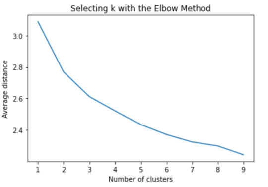
The elbow method suggest 2 or 3 clusters according to the graph
To plot the clusters, we need to reduce the variables, hence we transform the current variables into a canonical variables
from sklearn.decomposition import PCA
pca_2 = PCA(2)
plot_columns = pca_2.fit_transform(clus_train)
plt.scatter(x=plot_columns[:,0], y=plot_columns[:,1], c=model3.labels_,)
plt.xlabel('Canonical variable 1')
plt.ylabel('Canonical variable 2')
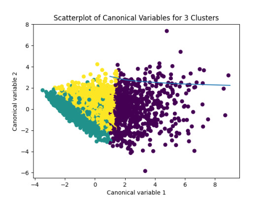
plt.title('Scatterplot of Canonical Variables for 3 Clusters')
plt.show()
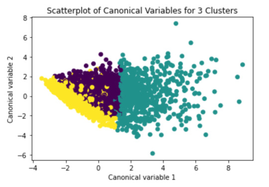
We can see a strong correlation between 2 clusters (Yellow & Purple)
Finally we group the clusters to evaluate the created model
clus_train.reset_index(level=0, inplace=True)
cluslist=list(clus_train['index'])
labels=list(model3.labels_)
newlist=dict(zip(cluslist, labels))
newlist
newclus=DataFrame.from_dict(newlist, orient='index')
newclus
newclus.columns = ['cluster']
newclus.reset_index(level=0, inplace=True)
merged_train=pd.merge(clus_train, newclus, on='index')
merged_train.head(n=100)
merged_train.cluster.value_counts()
This shows the elements by cluster
clustergrp = merged_train.groupby('cluster').mean()
print ("Clustering variable means by cluster")
print(clustergrp)
As we can see, Cluster 1 is strong in Marever 1 (use of marijuana) and Alcprobs1 (use of alcohol), on the other hand, cluster 2 is strong in Schconn (school connectedness) and Esteem1 (self esteem).
We can evaluate the relation between clusters
gpa_data=data_clean['GPA1']
gpa_train, gpa_test = train_test_split(gpa_data, test_size=.3, random_state=123)
gpa_train1=pd.DataFrame(gpa_train)
gpa_train1.reset_index(level=0, inplace=True)
merged_train_all=pd.merge(gpa_train1, merged_train, on='index')
sub1 = merged_train_all[['GPA1', 'cluster']].dropna()
import statsmodels.formula.api as smf
import statsmodels.stats.multicomp as multi
gpamod = smf.ols(formula='GPA1 ~ C(cluster)', data=sub1).fit()
print (gpamod.summary())
print ('means for GPA by cluster')
m1= sub1.groupby('cluster').mean()
print (m1)
print ('standard deviations for GPA by cluster')
m2= sub1.groupby('cluster').std()
print (m2)
mc1 = multi.MultiComparison(sub1['GPA1'], sub1['cluster'])
res1 = mc1.tukeyhsd()
print(res1.summary())

As we can see, the first table shows us data regarding the relationship between each cluster, which indicates that there is a considerable difference.
in the second table, we can see de GPA (Grade Point Average) is higher in cluster 2 where the features related to positive aspects regarding the use of alcohol and marijuana
0 notes
Text
Running a k-means Cluster Analysis
from pandas import Series, DataFrame
import pandas as pd
import numpy as np
import os
import matplotlib.pylab as plt
from sklearn.cross_validation import train_test_split
from sklearn.model_selection import train_test_split
from sklearn import preprocessing
from sklearn.cluster import KMeans
"""
Data Management
"""
os.chdir("C:\TREES")
data = pd.read_csv("tree_addhealth.csv")
upper-case all DataFrame column names
data.columns = map(str.upper, data.columns)
Data Management
data_clean = data.dropna()
subset clustering variables
cluster=data_clean[['ALCEVR1','MAREVER1','ALCPROBS1','DEVIANT1','VIOL1',
'DEP1','ESTEEM1','SCHCONN1','PARACTV', 'PARPRES','FAMCONCT']]
cluster.describe()
standardize clustering variables to have mean=0 and sd=1
clustervar=cluster.copy()
clustervar['ALCEVR1']=preprocessing.scale(clustervar['ALCEVR1'].astype('float64'))
clustervar['ALCPROBS1']=preprocessing.scale(clustervar['ALCPROBS1'].astype('float64'))
clustervar['MAREVER1']=preprocessing.scale(clustervar['MAREVER1'].astype('float64'))
clustervar['DEP1']=preprocessing.scale(clustervar['DEP1'].astype('float64'))
clustervar['ESTEEM1']=preprocessing.scale(clustervar['ESTEEM1'].astype('float64'))
clustervar['VIOL1']=preprocessing.scale(clustervar['VIOL1'].astype('float64'))
clustervar['DEVIANT1']=preprocessing.scale(clustervar['DEVIANT1'].astype('float64'))
clustervar['FAMCONCT']=preprocessing.scale(clustervar['FAMCONCT'].astype('float64'))
clustervar['SCHCONN1']=preprocessing.scale(clustervar['SCHCONN1'].astype('float64'))
clustervar['PARACTV']=preprocessing.scale(clustervar['PARACTV'].astype('float64'))
clustervar['PARPRES']=preprocessing.scale(clustervar['PARPRES'].astype('float64'))
split data into train and test sets
clus_train, clus_test = train_test_split(clustervar, test_size=.3, random_state=123)
k-means cluster analysis for 1-9 clusters
from scipy.spatial.distance import cdist
clusters=range(1,10)
meandist=[]
for k in clusters:
model=KMeans(n_clusters=k)
model.fit(clus_train)
clusassign=model.predict(clus_train)
meandist.append(sum(np.min(cdist(clus_train, model.cluster_centers_, 'euclidean'), axis=1))
/ clus_train.shape[0])
"""
Plot average distance from observations from the cluster centroid
to use the Elbow Method to identify number of clusters to choose
"""
plt.plot(clusters, meandist)
plt.xlabel('Number of clusters')
plt.ylabel('Average distance')
plt.title('Selecting k with the Elbow Method')
Interpret 3 cluster solution
model3=KMeans(n_clusters=3)
model3.fit(clus_train)
clusassign=model3.predict(clus_train)
plot clusters
from sklearn.decomposition import PCA
pca_2 = PCA(2)
plot_columns = pca_2.fit_transform(clus_train)
plt.scatter(x=plot_columns[:,0], y=plot_columns[:,1], c=model3.labels_,)
plt.xlabel('Canonical variable 1')
plt.ylabel('Canonical variable 2')
plt.title('Scatterplot of Canonical Variables for 3 Clusters')
plt.show()
"""
BEGIN multiple steps to merge cluster assignment with clustering variables to examine
cluster variable means by cluster
"""
create a unique identifier variable from the index for the
cluster training data to merge with the cluster assignment variable
clus_train.reset_index(level=0, inplace=True)
create a list that has the new index variable
cluslist=list(clus_train['index'])
create a list of cluster assignments
labels=list(model3.labels_)
combine index variable list with cluster assignment list into a dictionary
newlist=dict(zip(cluslist, labels))
newlist
convert newlist dictionary to a dataframe
newclus=DataFrame.from_dict(newlist, orient='index')
newclus
rename the cluster assignment column
newclus.columns = ['cluster']
now do the same for the cluster assignment variable
create a unique identifier variable from the index for the
cluster assignment dataframe
to merge with cluster training data
newclus.reset_index(level=0, inplace=True)
merge the cluster assignment dataframe with the cluster training variable dataframe
by the index variable
merged_train=pd.merge(clus_train, newclus, on='index')
merged_train.head(n=100)
cluster frequencies
merged_train.cluster.value_counts()
"""
END multiple steps to merge cluster assignment with clustering variables to examine
cluster variable means by cluster
"""
FINALLY calculate clustering variable means by cluster
clustergrp = merged_train.groupby('cluster').mean()
print ("Clustering variable means by cluster")
print(clustergrp)
validate clusters in training data by examining cluster differences in GPA using ANOVA
first have to merge GPA with clustering variables and cluster assignment data
gpa_data=data_clean['GPA1']
split GPA data into train and test sets
gpa_train, gpa_test = train_test_split(gpa_data, test_size=.3, random_state=123)
gpa_train1=pd.DataFrame(gpa_train)
gpa_train1.reset_index(level=0, inplace=True)
merged_train_all=pd.merge(gpa_train1, merged_train, on='index')
sub1 = merged_train_all[['GPA1', 'cluster']].dropna()
import statsmodels.formula.api as smf
import statsmodels.stats.multicomp as multi
gpamod = smf.ols(formula='GPA1 ~ C(cluster)', data=sub1).fit()
print (gpamod.summary())
print ('means for GPA by cluster')
m1= sub1.groupby('cluster').mean()
print (m1)
print ('standard deviations for GPA by cluster')
m2= sub1.groupby('cluster').std()
print (m2)
mc1 = multi.MultiComparison(sub1['GPA1'], sub1['cluster'])
res1 = mc1.tukeyhsd()
print(res1.summary())
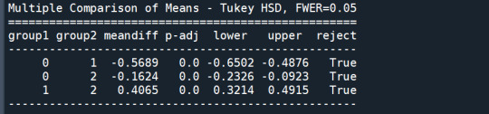
In order to externally validate the clusters, an Analysis of Variance (ANOVA) was conducting to test for significant differences between the clusters on grade point average (GPA). A tukey test was used for post hoc comparisons between the clusters. Results indicated significant differences between the clusters on GPA (F(3, 3197)=82.28, p<.0001). The tukey post hoc comparisons showed significant differences between clusters on GPA, with the exception that clusters 1 and 2 were not significantly different from each other. Adolescents in cluster 4 had the highest GPA (mean=2.99, sd=0.73), and cluster 3 had the lowest GPA (mean=2.42, sd=0.78).
0 notes
Text
Running a k-means Cluster Analysis
This post is the Machine Learning for Data Analysis week 3 Assignment.
Code
import pandas as pd
import numpy as np
import matplotlib.pyplot as plt
from sklearn import preprocessing
from sklearn.cluster import KMeans
snsdata = pd.read_csv("data.csv")
snsdata_clean = snsdata.dropna()
snsdata_clean.describe()
snsdata_clean['gender'] = preprocessing.LabelEncoder().fit_transform(snsdata_clean['gender'])
del snsdata_clean['gradyear'] # drop useless variable
for name in snsdata_clean.columns:
snsdata_clean[name] = preprocessing.scale(snsdata_clean[name]).astype('float64')
from scipy.spatial.distance import cdist
clusters = range(1,10)
meandist = []
for k in clusters:
model = KMeans(n_clusters = k,random_state = 123)
model.fit(snsdata_clean)
clusassign = model.predict(snsdata_clean)
meandist.append(sum(np.min(cdist(snsdata_clean,model.cluster_centers_,'euclidean'), axis = 1))/snsdata_clean.shape[0])
plt.plot(clusters, meandist)
plt.xlabel('Number of clusters')
plt.ylabel('Average distance')
plt.title('Selecting k with the Elbow Method')
plt.show()
from sklearn.decomposition import PCA
def kmeans(k):
model = KMeans(n_clusters = k,random_state = 123)
model.fit(snsdata_clean)
# plot clusters
pca_2 = PCA(2)
plot_columns = pca_2.fit_transform(snsdata_clean)
cols = ['r','g','b','y','m','c']
legentry = []
legkey = []
for i in range(k):
rowindex = model.labels_ == i
plot_ = plt.scatter(plot_columns[rowindex,0],plot_columns[rowindex,1], c = cols[i],)
exec('sc' + str(i) + " = plot_")
legentry.append(eval('sc' + str(i)))
legkey.append('Cluster ' + str(i + 1))
plt.legend(tuple(legentry),tuple(legkey),loc = 'lower right')
plt.xlabel('variable 1')
plt.ylabel('variable 2')
plt.title('Variables for ' + str(k) + ' Clusters')
plt.show()
kmeans(3)
model3 = KMeans(n_clusters = 3).fit(snsdata_clean)
snsdata_clean.reset_index(level = 0, inplace = True)
newclus = pd.DataFrame.from_dict(dict(zip(list(snsdata_clean['index']),list(model3.labels_))),orient = 'index')
newclus.columns = ['cluster']
newclus.reset_index(level = 0, inplace = True)
snsdata_merge = pd.merge(snsdata_clean,newclus, on = 'index')
#snsdata_merge.drop(snsdata_merge[['level_0','index']],axis=1, inplace=True)
snsdata_merge.cluster.value_counts()
clustergrp = snsdata_merge.groupby('cluster').mean()
print ("Clustering variable means by cluster")
print(clustergrp)
Output
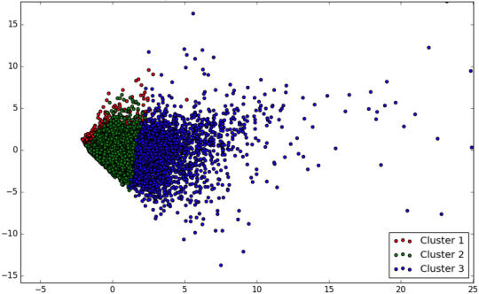
Interpretation
If we try with different number of clusters we can see that 3 has the largest number of observations.
Looking at the results, we see that compared to the other clusters, the variables in cluster 2 has levels on the culstering variables, meanwhile other variables shown in cluster 1 have high levels on the culstering variables.
0 notes
Text
Running a K-Means Cluster Analysis using Python
Python Code
# -- coding: utf-8 --
"""
Created on Mon Jan 18 19:51:29 2016
@author: jrose01
"""
from pandas import Series, DataFrame
import pandas as pd
import numpy as np
import matplotlib.pylab as plt
# from sklearn.cross_validation import train_test_split
from sklearn.model_selection import train_test_split
from sklearn import preprocessing
from sklearn.cluster import KMeans
"""
Data Management
"""
data = pd.read_csv("06.tree_addhealth.csv")
# upper-case all DataFrame column names
data.columns = map(str.upper, data.columns)
# Data Management
data_clean = data.dropna()
# subset clustering variables
cluster=data_clean[['ALCEVR1','MAREVER1','ALCPROBS1','DEVIANT1','VIOL1',
'DEP1','ESTEEM1','SCHCONN1','PARACTV', 'PARPRES','FAMCONCT']]
cluster.describe()
# standardize clustering variables to have mean=0 and sd=1
clustervar=cluster.copy()
clustervar['ALCEVR1']=preprocessing.scale(clustervar['ALCEVR1'].astype('float64'))
clustervar['ALCPROBS1']=preprocessing.scale(clustervar['ALCPROBS1'].astype('float64'))
clustervar['MAREVER1']=preprocessing.scale(clustervar['MAREVER1'].astype('float64'))
clustervar['DEP1']=preprocessing.scale(clustervar['DEP1'].astype('float64'))
clustervar['ESTEEM1']=preprocessing.scale(clustervar['ESTEEM1'].astype('float64'))
clustervar['VIOL1']=preprocessing.scale(clustervar['VIOL1'].astype('float64'))
clustervar['DEVIANT1']=preprocessing.scale(clustervar['DEVIANT1'].astype('float64'))
clustervar['FAMCONCT']=preprocessing.scale(clustervar['FAMCONCT'].astype('float64'))
clustervar['SCHCONN1']=preprocessing.scale(clustervar['SCHCONN1'].astype('float64'))
clustervar['PARACTV']=preprocessing.scale(clustervar['PARACTV'].astype('float64'))
clustervar['PARPRES']=preprocessing.scale(clustervar['PARPRES'].astype('float64'))
# split data into train and test sets
clus_train, clus_test = train_test_split(clustervar, test_size=.3, random_state=123)
# k-means cluster analysis for 1-9 clusters
from scipy.spatial.distance import cdist
clusters=range(1,10)
meandist=[]
for k in clusters:
model=KMeans(n_clusters=k)
model.fit(clus_train)
clusassign=model.predict(clus_train)
meandist.append(sum(np.min(cdist(clus_train,
model.cluster_centers_, 'euclidean'), axis=1))
/ clus_train.shape[0])
"""
Plot average distance from observations from the cluster centroid
to use the Elbow Method to identify number of clusters to choose
"""
plt.plot(clusters, meandist)
plt.xlabel('Number of clusters')
plt.ylabel('Average distance')
plt.title('Selecting k with the Elbow Method')
# Interpret 3 cluster solution
model3=KMeans(n_clusters=3)
model3.fit(clus_train)
clusassign=model3.predict(clus_train)
# plot clusters
from sklearn.decomposition import PCA
pca_2 = PCA(2)
plot_columns = pca_2.fit_transform(clus_train)
scatter = plt.scatter(x=plot_columns[:,0], y=plot_columns[:,1], c=model3.labels_)
plt.xlabel('Canonical variable 1')
plt.ylabel('Canonical variable 2')
plt.title('Scatterplot of Canonical Variables for 3 Clusters')
plt.legend(*scatter.legend_elements())
plt.show()
"""
BEGIN multiple steps to merge cluster assignment with clustering variables to examine
cluster variable means by cluster
"""
# create a unique identifier variable from the index for the
# cluster training data to merge with the cluster assignment variable
clus_train.reset_index(level=0, inplace=True)
# create a list that has the new index variable
cluslist=list(clus_train['index'])
# create a list of cluster assignments
labels=list(model3.labels_)
# combine index variable list with cluster assignment list into a dictionary
newlist=dict(zip(cluslist, labels))
newlist
# convert newlist dictionary to a dataframe
newclus=DataFrame.from_dict(newlist, orient='index')
newclus
# rename the cluster assignment column
newclus.columns = ['cluster']
# now do the same for the cluster assignment variable
# create a unique identifier variable from the index for the
# cluster assignment dataframe
# to merge with cluster training data
newclus.reset_index(level=0, inplace=True)
# merge the cluster assignment dataframe with the cluster training variable dataframe
# by the index variable
merged_train=pd.merge(clus_train, newclus, on='index')
merged_train.head(n=100)
# cluster frequencies
merged_train.cluster.value_counts()
"""
END multiple steps to merge cluster assignment with clustering variables to examine
cluster variable means by cluster
"""
# FINALLY calculate clustering variable means by cluster
clustergrp = merged_train.groupby('cluster').mean()
print ("Clustering variable means by cluster")
print(clustergrp)
# validate clusters in training data by examining cluster differences in GPA using ANOVA
# first have to merge GPA with clustering variables and cluster assignment data
gpa_data=data_clean['GPA1']
# split GPA data into train and test sets
gpa_train, gpa_test = train_test_split(gpa_data, test_size=.3, random_state=123)
gpa_train1=pd.DataFrame(gpa_train)
gpa_train1.reset_index(level=0, inplace=True)
merged_train_all=pd.merge(gpa_train1, merged_train, on='index')
sub1 = merged_train_all[['GPA1', 'cluster']].dropna()
import statsmodels.formula.api as smf
import statsmodels.stats.multicomp as multi
gpamod = smf.ols(formula='GPA1 ~ C(cluster)', data=sub1).fit()
print (gpamod.summary())
print ('means for GPA by cluster')
m1= sub1.groupby('cluster').mean()
print (m1)
print ('standard deviations for GPA by cluster')
m2= sub1.groupby('cluster').std()
print (m2)
mc1 = multi.MultiComparison(sub1['GPA1'], sub1['cluster'])
res1 = mc1.tukeyhsd()
print(res1.summary())
Output and Summary
A k-means cluster analysis was conducted to identify underlying subgroups of adolescents based on their similarity of responses on 11 variables that represent characteristics that could have an impact on school achievement. Clustering variables included two binary variables measuring whether or not the adolescent had ever used alcohol or marijuana, as well as quantitative variables measuring alcohol problems, a scale measuring engaging in deviant behaviors (such as vandalism, other property damage, lying, stealing, running away, driving without permission, selling drugs, and skipping school), and scales measuring violence, depression, self-esteem, parental presence, parental activities, family connectedness, and school connectedness. All clustering variables were standardized to have a mean of 0 and a standard deviation of 1.
Data were randomly split into a training set that included 70% of the observations (N=3202) and a test set that included 30% of the observations (N=1373). A series of k-means cluster analyses were conducted on the training data specifying k=1-9 clusters, using Euclidean distance. The average minimum distance value in the observation to the cluster centroids was plotted for each of the nine cluster solutions in an elbow curve to provide guidance for choosing the number of clusters to interpret.

The elbow curve was inconclusive, suggesting that the 2 and 3-cluster solutions might be interpreted. The results below are for an interpretation of the 3-cluster solution.
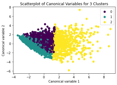
Canonical discriminant analyses was used to reduce the 11 clustering variable down a few variables that accounted for most of the variance in the clustering variables. A scatterplot of the first two canonical variables by cluster (Figure 2 shown below) indicated that the observations in clusters 0 and 1 were densely packed with relatively low within cluster variance, and did not overlap very much with the other clusters. Observations in cluster 2 were spread out more than the other clusters, showing high within cluster variance. The results of this plot suggest that the best cluster solution may have fewer than 3 clusters, so it will be especially important to also evaluate the cluster solutions with fewer than 3 clusters.
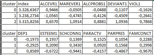
The means on the clustering variables showed that, compared to the other clusters, adolescents in cluster 1 were the least troubled. Compared to adolescents in the other clusters, they were least likely to have used alcohol and marijuana, and had the lowest number of alcohol problems, and deviant and violent behavior. They also had the lowest levels of depression, and higher self-esteem, school connectedness, parental presence and family connectedness and one of the highest for parental involvement in activities. On the other hand, cluster 2 clearly included the most troubled adolescents. Adolescents in cluster 2 had a very high likelihood of having used alcohol, the highest likelihood of having used marijuana, more alcohol problems, and more engagement in deviant and violent behaviors compared to the other clusters. They also had higher levels of depression, and the lowest levels of self-esteem, school connectedness, parental presence, involvement of parents in activities, and family connectedness. Adolescents in cluster 1 had moderate values except for the likelyhood of having used alcohol and school connectedness, which are the highest.
In order to externally validate the clusters, an Analysis of Variance (ANOVA) was conducting to test for significant differences between the clusters on grade point average (GPA). A tukey test was used for post hoc comparisons between the clusters. Results indicated significant differences between the clusters on GPA. The tukey post hoc comparisons showed significant differences between clusters on GPA, with the exception that clusters 0 and 1 were not significantly different from each other. Adolescents in cluster 2 had the lowest GPA (mean=2.42, sd=0.78).
0 notes
Text

13 clouds, 7 briefcases, new album/music on 13th July? 💖🦋 @taylorswift @taylornation #taylorswift
8 notes
·
View notes
Text
Rock Mania Rises Again Playlist hosted by Jacqueline Jax
TODAY'S LIST OF WHAT'S FRESH COMING INTO A.V.A LIVE RADIO. THIS IS A ROCK GENRE SHOW SEGMENT FULL OF MUSIC THAT WILL INSPIRE YOU AND SEND YOU SEARCHING THE ARTISTS PAGES FOR MORE. EPISODE HOSTED BY JACQUELINE JAX.
Todays show is all about Rock and Roll. Get ready Rock fans to discover some new favorites.
Listen to the show : 2 pm et : https://anchor.fm/ava-live-radio
FEATURED ARTISTS:
Artist: Beautiful Things
New Release: Hey Hey Hey (Electric Mix)
Genre: Alternative Rock
Sounds like: Garbage, Placebo, Curve
Located in: Los Angeles, CA
Our band creates ethereal pop-rock with deeply personal lyrics. I wrote this song about my experiences with the music industry, looking back to a time when I was much younger and more trusting. I let people guide me and represent me who didn’t have my best interests at heart – only their own. I learned so much from these experiences about human nature which ultimately strengthened me and made me a smarter, wiser person.
I wanted this song to be empowering, hence the lyric “I won’t be a victim, no never again.” I’ve since chosen the people I surround myself within all areas of my life very carefully and have learned to trust my intuition. It’s made all the difference. Our new Dream World (Revisited) EP is made up of re-imagined songs from the first Beautiful Things album released 10 years ago, called just Dream World. We are working on a new single and will be making a video to promote it.
LINKS:
https://open.spotify.com/track/0G9QeybSCD1SYCIpr6vrA6
https://twitter.com/officialthings
https://www.facebook.com/beautifulthingsmusic
https://www.instagram.com/beautifulthingsmusic
Artist: Dream Eternal Bliss
New Release: Circling
Genre: alternative rock
Sounds like: Berlin, The Cardigans, Garbage, Duran Duran
Located in: Franklin Lakes, NJ
This song is a moody ballad about your life being stuck in a holding pattern. Challenges we face tend to provide great songwriting material when you want to craft truly personal and heartfelt lyrics. If you’ve ever felt like time is passing you by and you’re sort of immobilized by your situation, powerless to take control and make a change, whether it’s a relationship or work or something else, that’s exactly where “Circling" came from. I find that the happiest times in my life are the most challenging times in which to write personal lyrics.
This song encapsulates a variety of musical influences. It starts with a synth-meets-U2 vibe over some electronic percussion that evolves into something dark and somber, and then in the second half, big drums and heavy guitar kick in. Right now we are shooting a video for this song!
LINKS:
https://www.reverbnation.com/dreameternalbliss/song/30421617-circling
https://open.spotify.com/track/1cqQihDUv9ZInj9Qpeh9jh
https://www.facebook.com/dreameternalbliss
https://www.instagram.com/dreameternalbliss
Artist: Ugly Melon
New Release: Rainbow in the Dark
Genre: Hard rock / Metal /Rock /
Sounds like: Black Sabbath / Disturbed / Shinedown
Located in: Toronto Ontario Canada
Ugly Melon comes from an era of classic hard rock from the 70s Black Sabbath to today modern edge of Disturbed. 'Rainbow in the dark' is a song written by Ronnie James Dio back in 1983 from the Holy Diver album, the Original song was an up yet simple song. We put our Ugly Melon twist to it and made the song a more Modern ballad anthem. The feeling of being alone and rejected but you are really a rainbow in the dark. When doing such an epic song like this that was a huge hit for Dio, you've got to make sure you don't butcher the song. Our new album 'Just a Man' is a piece of work we are proud of and love hearing it every time.
Ugly Melon will be releasing a video soon probably on Halloween song called 'If You're Wrong'. A song about questioning and challenging religious beliefs and to be open-minded to others beliefs.
LINKS:
https://www.reverbnation.com/uglymelon/song/30535606-rainbow-in-the-dark
https://open.spotify.com/track/6jkS0MMp6jl45iyjO3xNE5?si=6aXL5FW2QrWHm_ofcGZ7Iw
https://twitter.com/Ugly_Melon
https://www.facebook.com/uglymelon
Instagram @Ugly_Melon
Artist: Jet Set Future
New Release: VICE
Genre: Alternative, Indie-Rock, Post-hardcore
Sounds like: : Best Coast, Pvris, No Doubt, Bloxx, Wavves, Foo Fighters, Paramore
Located in: Plymouth, Massachusetts United States of America
This song is a nice Blending of Beautiful vocal melodies with a Lead bass, loud drums, and powerful catchy guitars. This song, in particular, has a post-hardcore, chill feel. It's about waiting for the right person to come along, and all of the struggles, and heartache that comes before it. This release is important to our music direction because it shows you a foreshadowing of what's to come on our Full Length. But without giving you too many details. We can be poppy and peppy. We can be dark, we can have a feeling like you're relaxing on a beach, we can also add a sense of classical. As of now we're finishing up and putting our final tweaks onto our first Full-Length album. Next, we will be working on a music video for our next single.
LINKS:
https://www.reverbnation.com/jetsetfuture/song/31128331-vice
https://open.spotify.com/track/2kja9ILXtyiaXRbsojRIog?si=xFs7SXFdSrepvLc5N8qu4g
http://www.twitter.com/jetsetfuture4
https://www.facebook.com/JetSetFuture
https://www.instagram.com/JetSetFutureBand
Artist: Population U
New Release: Now you see
Genre: Alt Rock, Indie Rock, alternative, emo
Sounds like: Offspring, Green Day, rise against
Located in: Anaheim, Ca USA
'Now you see' is not just a song about a breakup or losing someone you love, it's a song about realizing your self-value after it's over. The song showcases our songwriting and it is one of our favorite songs to perform. We are releasing this single with a Music Video to showcase our Stage Show With our PopU Dancers. We are focusing on a Stage show for the New Year. With a year in preparation behind us to create an alternative rock stage show that incorporates actual Dancers with the music, it's time to get the ball rolling. Right now we just finished a video for our single "Now you see" and will be releasing it on our YouTube channel. We have a few more videos to shoot and we have 2 shows with our dancers. By the beginning of next year, the band will start recording more singles.
LINKS:
https://twitter.com/populationu
https://open.spotify.com/artist/02vPDEV6Eqm4tbozbKDNHL
https://soundcloud.com/population-u
https://www.reverbnation.com/populationu
https://www.instagram.com/populationumusic
https://www.facebook.com/populationu
Artist: Black Rose Reception
New Release: Up jumped the devil
Genre: Hard rock
Sounds like: Judas Priest, Iron Maiden
Located in: Indiana
The music we are creating is old and new school music mix. The message in this song is you can overcome the demons of depression, suicide, and stress that we all deal with. There are great and professional people out there who can help so never feel embarrassed to ask fo help. Right now we are going in studio recording more new tracks.
LINKS:
https://open.spotify.com/album/0HEOkTc5fXQyYCr1jwFSeF
https://twitter.com/blackroserecept
https://www.facebook.com/BlackRoseReceptionMusic
https://www.instagram.com/blackrosereceptio
https://store.cdbaby.com/Artist/BlackRoseReception
Artist: NewClue
New Release: Hail to the King (Henry VIII)
Genre: Nostalgic Metal Reborn
Sounds like: : AC/DC, Iron Maiden, Megadeth, XYZ, Dio, Queenrych,
Nostalgic Metal bands.
Located in: New London CT, USA
Nostalgic Metal Reborn with a NewClue. This is a biography of the life of King Henry VIII with some GREAT guitar leads!
The music we are creating is NOSTALGIC METAL REBORN. As formed in the very late '80s as NoClue and after about 7 years, went our separate ways. We Reformed into NewClue in 2014, which has won many awards and put us into rotation on many radio stations worldwide.
With many of the yester-year's 80's and 90's rock bands on tour today and all of the tribute bands going over like Blockbusters, it's the perfect time to catch a NewClue.
Right now with all the mania alive towards classic rock bands and the Tribute bands on the circuit, we are creating a Godsmack tribute band. Of course, NewClue will always be the opening act!
LINKS:
REVERBNATION: www.reverberation.com/newclue
SPOTIFY: https://open.spotify.com/user/22kksixsltmqrozubnt3xytoa/playlist/01MSrnctE7bm1Qs7VhHgHt?si=MY3PWLymQuepRp90nTHJCA
TWITTER: www.twitter.com/NewClue2
FACEBOOK: www.facebook.com/NewClueBand
INSTAGRAM: www.instagram.com/neil.whittington
Our favorite: Number One Music: www.numberonemusic.com/newclue
Artist: David Bucci
New Release: Dangerous
Genre: Indie Alternative Rock
Sounds like: Bon Jovi, Chris Stapleton, Bryan Adams, Ritchie Kotzen, Goo Goo Dolls, Keith Urban
Located in: Channel Islands, Ca
When asked to describe his new release in a few words, David Bucci said, "Dirty boots, blue-collar, indie alternative rock music. Dangerous, off the new album, Country Club." 'Dangerous' has a heavy acoustic guitar and drum-driven influence with electric guitar layers and soling over it along with my lead vocals and backup harmonies by Robert Cross. The message behind ‘Dangerous’ is a sort of realistic caution about life, that we can be derailed very easily and things can spiral quickly. We need to take care of ourselves and don’t put ourselves in bad positions and places.
Right now we are preparing for the album's release, planning a new music video. Tour, not yet, local clubs and bars at the moment, but who knows, arenas and stadiums may be right around the corner.
LINKS:
Website http://www.david-bucci.com
Spotify https://open.spotify.com/artist/0SFT53gEfnxneyzaEvgEGK
Instagram: https://www.instagram.com/davidbucci_official
Facebook https://m.facebook.com/thedavidbucciofficial
Twitter https://mobile.twitter.com/DgbBucci
Artist: The Yellow Jacks
New Release: Georgia Peach
Genre: Rock, Blues Rock , Psychedelic Rock, Country Rock
Sounds like: : Led Zeppelin, The Rolling Stones, Cream, The Beatles, The Black Keys, Wolfmother and The Artic Monkeys
Located in: Long Island, New York United States
This is a song about a couple of guys from New York going to Georgia. Four piece energetic, soulful original rock band inspired by classic rock bands such as Led Zeppelin, Cream and The Rolling Stones. We are also inspired by modern rock bands like The Black Keys, Artic Monkeys and Wolfmother. We just released our debut album entitled From The Ashes and want to keep growing our discography by releasing new music and playing live shows. Music is our passion and we want to touch people's hearts with our songs and performances.
LINKS:
Spotify: https://open.spotify.com/album/0BNflbZX7Nj00NaylB5PXk?si=XLcv8mzfSUSqRN_bTvNoHw
The Yellow Jacks (@TheYellowJacks): https://twitter.com/TheYellowJacks
https://www.facebook.com/theyellowjacksLI
https://www.instagram.com/the_yellow_jacks
Artist: Shehzad Bhanji - Instrumental Guitarist
New Release: Matched Hearts
Genre: Instrumental Rock, Melodic Rock, Soft Rock, Pop Rock
Sounds like: Lady Antebellum (for the new song Matched Hearts) and Joe Satriani
Joe Satriani (For the majority of the tracks)
Located in: Doha Qatar
‘Matched Hearts’ is an anthem that describes deep and intimate love as two people’s hearts being in sync with each other. The song is about celebrating the different moments that come with love unedited and completely raw: from moments of desperation to moments of pure bliss. I'm an instrumental rock guitarist whose powerful melodies have touched millions of hearts. Matched Hearts is the first release from my 3rd Album DREAMS. I’m releasing a music video of Matched Hearts, which will provide the launchpad for the release of my 3rd solo instrumental album.
LINKS:
Presave the Album: http://bit.ly/shehzadbhanji
New Music Video: http://bit.ly/matchedhearts
Website: www.shehzadbhanji.com
Soundcloud: https://soundcloud.com/shehzad-bhanji/matchedhearts/s-dVnAP
Instagram: https://www.instagram.com/shehzadbhanji
Facebook: https://www.facebook.com/shehzad.bhanji
Twitter: https://twitter.com/ShehzadBhanji
Artist: Graham Greene
New Release: Night of the Djinn
Genre: Symphonic Metal - Instrumental
Sounds like: Nightwish, Kamelot, Trans Siberian Orchestra, Joe Satriani,
Located in: Perth, Western Australia
A symphonic blend of Eastern, Classical and Metal to conjure images of the mystical Orient. Orchestration meets heavy guitars to tell the Djinn's tale. This song flowed from beginning to end in the writing and recording process, and I found myself caught up in the story as I went. Sometimes you write the song, and sometimes the song writes you. New videos are in the planning to promote the new album, "A Ripple in Time", which is now online in all the best places.
LINKS:
https://open.spotify.com/track/0KvqWl95ymm8mUhsCtzlmp?si=bcPCG25LReO4aPhRyiaEUA
https://www.facebook.com/GrahamGreeneGuitarist
https://twitter.com/Graham_Greene
https://www.instagram.com/grahamgreeneguitarist
Artist: Dave Molter
New Release: Tell Me That You Love Me
Genre: Rock
Sounds like: Beatles, Byrds, Searchers
Located in: Pittsburgh, PA USA
An accomplished veteran of the East Coast and Midwest music scene, Dave Molter counts the Beatles as his primary Influence. His latest single "Tell Me That You Love Me" is a tribute to the Fab Four and the British Invasion era, when getting the attention of someone you loved was the moving force for young people. It has Beatlesque harmonies and tone as well as the 12-string jangle of the Beatles, Byrds, Holliea, and Searchers. It's a happy song! "Tell Me That You Love Me is one of five songs on my debut EP, "Foolish Heart." Right now I'm excited to continue working on a full CD, which we hope will be available in early 2020.
LINKS:
https://www.reverbnation.com/davemolter/song/31091471-04-tell-me-that-you-love-me
Twitter: @molter_dave
www.facebook.com/davemoltermusic
Instagram: @davemolter
Artist: Vovkulaka
New Release: my Devil
Genre: Metal/Dubstep
Located in: Odessa, Ukraine
Music creator from Odessa composing music that investigates the unusual.
Have you ever been in a relationship where you find yourself doing things that normally, you never do? The situation almost possesses you to struggle but still, you can't manage to break away. The desire is the conundrum. Like Demons with thoughts... A living Hell. You stop and think this is my Devil.
The music we are creating is Dark... Angry... Evil... Metal
Right now we are preparing to release our CD.
LINKS:
Spotify: https://open.spotify.com/album/3928niLRX3PB1EbxuRvhpu?si=OSLSKd0JRA-g8eghCufsrQ
Twitter: Twitter.com/VovkulakaMusic
Facebook: Facebook.com/VovkulakaFanPage
Instagram: Instagram.com/VovkulakaMusic
Artist: Collins & Streiss
New Release: Freedom's Captive
Genre: Rock, Commercial Rock, Indie Rock, Alternative Rock
Located in: Richmond Hill, Ontario, Canada
"Freedom's Captive" is about our growing addiction to our devices, whether it's cell phones, computers, tablets, social media and so on, and this obsession and need for acquiring followers and likes in today's web of virtual existence. It's a compounding obsession in a lot of cases where we have all this freedom and ability to exist and do what we want virtually now, but at the same time are becoming captives to it! This song involves a few other players and has more of an overall band feel to it. The song is upbeat, edgy and energetic and full of catchy melodies and hooks which is common in our music. It's derivative of our rock roots which has a broad range of artists and rich heritage.
LINKS:
Reverbnation: https://www.reverbnation.com/collinsandstreiss
Spotify: https://open.spotify.com/album/2zOmvGgES8y4jvKtzVGOa3
Twitter: https://twitter.com/collins_streiss
Facebook: https://www.facebook.com/Collins-and-Streiss-762369407204284
Instagram: https://www.instagram.com/collins_and_streiss
FOLLOW OUR PLAYLIST
#Rock Music#metal#Beautiful Things#Dream Eternal Bliss#Ugly Melon#Jet Set Future#Population U#Black Rose Reception#NewClue#David Bucci#The Yellow Jacks#Shehzad Bhanji#Graham Greene#Dave Molter#Vovkulaka#Collins & Streiss
0 notes
Text
Week 4 - KMean Cluster
Please find below the source code, console output and plot based on KMean Cluster analysis. Kindly review the same ASAP. Thanks
SOURCE CODE
# -*- coding: utf-8 -*-
“”“
Created on Mon Jan 18 19:51:29 2016
@author: sundar
”“”
from pandas import Series, DataFrame
import pandas as pd
import numpy as np
import matplotlib.pylab as plt
from sklearn.model_selection import train_test_split
from sklearn import preprocessing
from sklearn.cluster import KMeans
“”“
Data Management
”“”
data = pd.read_csv(“tree_addhealth.csv”)
#upper-case all DataFrame column names
data.columns = map(str.upper, data.columns)
# Data Management
data_clean = data.dropna()
# subset clustering variables
cluster=data_clean[[‘ALCEVR1’,'MAREVER1’,'ALCPROBS1’,'DEVIANT1’,'VIOL1’,
'DEP1’,'ESTEEM1’,'SCHCONN1’,'PARACTV’, 'PARPRES’,'FAMCONCT’]]
cluster.describe()
# standardize clustering variables to have mean=0 and sd=1
clustervar=cluster.copy()
clustervar['ALCEVR1’]=preprocessing.scale(clustervar['ALCEVR1’].astype('float64’))
clustervar['ALCPROBS1’]=preprocessing.scale(clustervar['ALCPROBS1’].astype('float64’))
clustervar['MAREVER1’]=preprocessing.scale(clustervar['MAREVER1’].astype('float64’))
clustervar['DEP1’]=preprocessing.scale(clustervar['DEP1’].astype('float64’))
clustervar['ESTEEM1’]=preprocessing.scale(clustervar['ESTEEM1’].astype('float64’))
clustervar['VIOL1’]=preprocessing.scale(clustervar['VIOL1’].astype('float64’))
clustervar['DEVIANT1’]=preprocessing.scale(clustervar['DEVIANT1’].astype('float64’))
clustervar['FAMCONCT’]=preprocessing.scale(clustervar['FAMCONCT’].astype('float64’))
clustervar['SCHCONN1’]=preprocessing.scale(clustervar['SCHCONN1’].astype('float64’))
clustervar['PARACTV’]=preprocessing.scale(clustervar['PARACTV’].astype('float64’))
clustervar['PARPRES’]=preprocessing.scale(clustervar['PARPRES’].astype('float64’))
# split data into train and test sets
clus_train, clus_test = train_test_split(clustervar, test_size=.3, random_state=123)
# k-means cluster analysis for 1-9 clusters
from scipy.spatial.distance import cdist
clusters=range(1,10)
meandist=[]
for k in clusters:
model=KMeans(n_clusters=k)
model.fit(clus_train)
clusassign=model.predict(clus_train)
meandist.append(sum(np.min(cdist(clus_train, model.cluster_centers_, 'euclidean’), axis=1))
/ clus_train.shape[0])
“”“
Plot average distance from observations from the cluster centroid
to use the Elbow Method to identify number of clusters to choose
”“”
plt.plot(clusters, meandist)
plt.xlabel('Number of clusters’)
plt.ylabel('Average distance’)
plt.title('Selecting k with the Elbow Method’)
# Interpret 3 cluster solution
model3=KMeans(n_clusters=3)
model3.fit(clus_train)
clusassign=model3.predict(clus_train)
# plot clusters
from sklearn.decomposition import PCA
pca_2 = PCA(2)
plot_columns = pca_2.fit_transform(clus_train)
plt.scatter(x=plot_columns[:,0], y=plot_columns[:,1], c=model3.labels_,)
plt.xlabel('Canonical variable 1’)
plt.ylabel('Canonical variable 2’)
plt.title('Scatterplot of Canonical Variables for 3 Clusters’)
plt.show()
“”“
BEGIN multiple steps to merge cluster assignment with clustering variables to examine
cluster variable means by cluster
”“”
# create a unique identifier variable from the index for the
# cluster training data to merge with the cluster assignment variable
clus_train.reset_index(level=0, inplace=True)
# create a list that has the new index variable
cluslist=list(clus_train['index’])
# create a list of cluster assignments
labels=list(model3.labels_)
# combine index variable list with cluster assignment list into a dictionary
newlist=dict(zip(cluslist, labels))
newlist
# convert newlist dictionary to a dataframe
newclus=DataFrame.from_dict(newlist, orient='index’)
newclus
# rename the cluster assignment column
newclus.columns = ['cluster’]
# now do the same for the cluster assignment variable
# create a unique identifier variable from the index for the
# cluster assignment dataframe
# to merge with cluster training data
newclus.reset_index(level=0, inplace=True)
# merge the cluster assignment dataframe with the cluster training variable dataframe
# by the index variable
merged_train=pd.merge(clus_train, newclus, on='index’)
merged_train.head(n=100)
# cluster frequencies
merged_train.cluster.value_counts()
“”“
END multiple steps to merge cluster assignment with clustering variables to examine
cluster variable means by cluster
”“”
# FINALLY calculate clustering variable means by cluster
clustergrp = merged_train.groupby('cluster’).mean()
print (“Clustering variable means by cluster”)
print(clustergrp)
# validate clusters in training data by examining cluster differences in GPA using ANOVA
# first have to merge GPA with clustering variables and cluster assignment data
gpa_data=data_clean['GPA1’]
# split GPA data into train and test sets
gpa_train, gpa_test = train_test_split(gpa_data, test_size=.3, random_state=123)
gpa_train1=pd.DataFrame(gpa_train)
gpa_train1.reset_index(level=0, inplace=True)
merged_train_all=pd.merge(gpa_train1, merged_train, on='index’)
sub1 = merged_train_all[['GPA1’, 'cluster’]].dropna()
import statsmodels.formula.api as smf
import statsmodels.stats.multicomp as multi
gpamod = smf.ols(formula='GPA1 ~ C(cluster)’, data=sub1).fit()
print (gpamod.summary())
print ('means for GPA by cluster’)
m1= sub1.groupby('cluster’).mean()
print (m1)
print ('standard deviations for GPA by cluster’)
m2= sub1.groupby('cluster’).std()
print (m2)
mc1 = multi.MultiComparison(sub1['GPA1’], sub1['cluster’])
res1 = mc1.tukeyhsd()
print(res1.summary())
CONSOLE
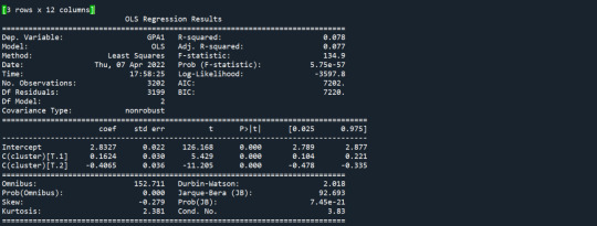
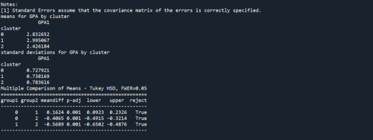
PLOT OUTPUT
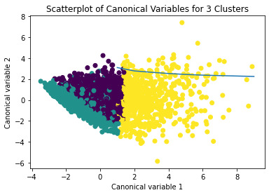
ANALYSIS
3 adolescents in the cluster were considered for analysis:-
Cluster 0 - highest likelihood of having used alcohol
Cluster 1 - Most troubled adolescents
Cluster 2 - Least troubled adolescents
As a part of the analysis, it was observed that adolescents in cluster (the most troubled group) had the lowest GPA of 2.44; adolescents in cluster 2 (least troubled group, had the highest GPA of 3.01.
As a part of the tukey test, it was observed that the clusters differed significantly in mean GPA, although the difference between cluster 0 and cluster 2 were smaller.
0 notes
Text
Week 4 K-Cluster Analysis
from pandas import Series, DataFrame
import pandas as pd
import numpy as np
import matplotlib.pylab as plt
from sklearn.model_selection import train_test_split
from sklearn import preprocessing
from sklearn.cluster import KMeans
import os
file = open(os.path.expanduser("~/Desktop/TreeAddHealth.csv"))
# Load and manage data
AH_data = pd.read_csv(file)
AH_data.columns = map(str.upper, AH_data.columns)
data_clean = AH_data.dropna()
# subset clustering variables
cluster = data_clean[['ALCEVR1', 'MAREVER1', 'ALCPROBS1', 'DEVIANT1', 'VIOL1',
'DEP1', 'ESTEEM1', 'SCHCONN1', 'PARACTV', 'PARPRES', 'FAMCONCT']]
cluster.describe()
# standardize clustering variables to have mean=0 & sd=1
clustervar = cluster.copy()
clustervar['ALCEVR1'] = preprocessing.scale(clustervar['ALCEVR1'].astype('float64'))
clustervar['ALCPROBS1'] = preprocessing.scale(clustervar['ALCPROBS1'].astype('float64'))
clustervar['MAREVER1'] = preprocessing.scale(clustervar['MAREVER1'].astype('float64'))
clustervar['DEP1'] = preprocessing.scale(clustervar['DEP1'].astype('float64'))
clustervar['ESTEEM1'] = preprocessing.scale(clustervar['ESTEEM1'].astype('float64'))
clustervar['VIOL1'] = preprocessing.scale(clustervar['VIOL1'].astype('float64'))
clustervar['DEVIANT1'] = preprocessing.scale(clustervar['DEVIANT1'].astype('float64'))
clustervar['FAMCONCT'] = preprocessing.scale(clustervar['FAMCONCT'].astype('float64'))
clustervar['SCHCONN1'] = preprocessing.scale(clustervar['SCHCONN1'].astype('float64'))
clustervar['PARACTV'] = preprocessing.scale(clustervar['PARACTV'].astype('float64'))
clustervar['PARPRES'] = preprocessing.scale(clustervar['PARPRES'].astype('float64'))
# split data in train & test sets
clus_train, clus_test, = train_test_split(clustervar, test_size=.3, random_state=123)
# k-means cluster analysis for 1-9 clusters
from scipy.spatial.distance import cdist
clusters = range(1, 10)
meandist = []
for k in clusters:
model = KMeans(n_clusters=k)
model.fit(clus_train)
clusassign = model.predict(clus_train)
meandist.append(sum(np.min(cdist(clus_train, model.cluster_centers_, 'euclidean'), axis=1)))
# plt.plot(clusters, meandist) >> comment out to hide
plt.xlabel('Number of clusters')
plt.ylabel('Average distance')
plt.title('Selecting k with the Elbow method')
# Interpret 3 cluster solution
model3 = KMeans(n_clusters=3)
model3.fit(clus_train)
clusassign = model3.predict(clus_train)
# plot clusters
from sklearn.decomposition import PCA
pca_2 = PCA(2)
plot_columns = pca_2.fit_transform(clus_train)
plt.scatter(x=plot_columns[:, 0], y=plot_columns[:, 1], c=model3.labels_)
plt.xlabel('Canonical variable 1')
plt.ylabel('Canonical variable 2')
plt.title('Scatterplot of Canonical Variables for 3 Clusters')
# plt.show()
# create a unique identifier variable from the index
clus_train.reset_index(level=0, inplace=True)
# create a list for the new index variable
cluslist = list(clus_train['index'])
# create a list of cluster assignments
labels = list(model3.labels_)
# combine index variable list with cluster assignment list into a dictionary, dataframe
newlist = dict(zip(cluslist, labels))
newlist
newclus = DataFrame.from_dict(newlist, orient='index')
newclus
newclus.columns = ['cluster']
newclus.reset_index(level=0, inplace=True)
merged_train = pd.merge(clus_train, newclus, on='index')
merged_train.head(n=100)
# cluster frequencies
merged_train.cluster.value_counts()
# calculate clustering variable means by cluster
clustergrp = merged_train.groupby('cluster').mean()
# print("Clustering variable means by cluster")
# print(clustergrp)
# validate clusters in training data
gpa_data = data_clean['GPA1']
# create train & test sets
gpa_train, gpa_test = train_test_split(gpa_data, test_size=.3, random_state=123)
gpa_train1 = pd.DataFrame(gpa_train)
gpa_train1.reset_index(level=0, inplace=True)
merged_train_all = pd.merge(gpa_train1, merged_train, on='index')
sub1 = merged_train_all[['GPA1', 'cluster']].dropna()
import statsmodels.formula.api as smf
import statsmodels.stats.multicomp as multi
gpamod = smf.ols(formula='GPA1 ~ C(cluster)', data=sub1).fit()
print(gpamod.summary())
print('means for GPA by cluster')
m1 = sub1.groupby('cluster').mean()
print(m1)
print('Standard deviations for GPA by cluster')
m2 = sub1.groupby('cluster').std()
print(m2)
mc1 = multi.MultiComparison(sub1['GPA1'], sub1['cluster'])
res1 = mc1.tukeyhsd()
print(res1.summary)
OUTPUT:
OLS Regression Results
==============================================================================
Dep. Variable: GPA1 R-squared: 0.077
Model: OLS Adj. R-squared: 0.076
Method: Least Squares F-statistic: 133.3
Date: Wed, 11 May 2022 Prob (F-statistic): 2.50e-56
Time: 18:48:25 Log-Likelihood: -3599.3
No. Observations: 3202 AIC: 7205.
Df Residuals: 3199 BIC: 7223.
Df Model: 2
Covariance Type: nonrobust
===================================================================================
coef std err t P>|t| [0.025 0.975]
-----------------------------------------------------------------------------------
Intercept 2.9945 0.020 151.472 0.000 2.956 3.033
C(cluster)[T.1] -0.5685 0.035 -16.314 0.000 -0.637 -0.500
C(cluster)[T.2] -0.1646 0.030 -5.512 0.000 -0.223 -0.106
==============================================================================
Omnibus: 154.326 Durbin-Watson: 2.019
Prob(Omnibus): 0.000 Jarque-Bera (JB): 92.624
Skew: -0.277 Prob(JB): 7.71e-21
Kurtosis: 2.377 Cond. No. 3.41
==============================================================================
Notes:
[1] Standard Errors assume that the covariance matrix of the errors is correctly specified.
means for GPA by cluster
GPA1
cluster
0 2.994542
1 2.426063
2 2.829949
Standard deviations for GPA by cluster
GPA1
cluster
0 0.738174
1 0.786903
2 0.727230
<bound method TukeyHSDResults.summary of <statsmodels.sandbox.stats.multicomp.TukeyHSDResults object at 0x157a87520>>
Process finished with exit code 0
0 notes
Text
Week 4 - KMean Cluster
Please find below the source code, console output and plot based on KMean Cluster analysis. Kindly review the same ASAP. Thanks
SOURCE CODE
# -*- coding: utf-8 -*-
"""
Created on Mon Jan 18 19:51:29 2016
@author: sundar
"""
from pandas import Series, DataFrame
import pandas as pd
import numpy as np
import matplotlib.pylab as plt
from sklearn.model_selection import train_test_split
from sklearn import preprocessing
from sklearn.cluster import KMeans
"""
Data Management
"""
data = pd.read_csv("tree_addhealth.csv")
#upper-case all DataFrame column names
data.columns = map(str.upper, data.columns)
# Data Management
data_clean = data.dropna()
# subset clustering variables
cluster=data_clean[['ALCEVR1','MAREVER1','ALCPROBS1','DEVIANT1','VIOL1',
'DEP1','ESTEEM1','SCHCONN1','PARACTV', 'PARPRES','FAMCONCT']]
cluster.describe()
# standardize clustering variables to have mean=0 and sd=1
clustervar=cluster.copy()
clustervar['ALCEVR1']=preprocessing.scale(clustervar['ALCEVR1'].astype('float64'))
clustervar['ALCPROBS1']=preprocessing.scale(clustervar['ALCPROBS1'].astype('float64'))
clustervar['MAREVER1']=preprocessing.scale(clustervar['MAREVER1'].astype('float64'))
clustervar['DEP1']=preprocessing.scale(clustervar['DEP1'].astype('float64'))
clustervar['ESTEEM1']=preprocessing.scale(clustervar['ESTEEM1'].astype('float64'))
clustervar['VIOL1']=preprocessing.scale(clustervar['VIOL1'].astype('float64'))
clustervar['DEVIANT1']=preprocessing.scale(clustervar['DEVIANT1'].astype('float64'))
clustervar['FAMCONCT']=preprocessing.scale(clustervar['FAMCONCT'].astype('float64'))
clustervar['SCHCONN1']=preprocessing.scale(clustervar['SCHCONN1'].astype('float64'))
clustervar['PARACTV']=preprocessing.scale(clustervar['PARACTV'].astype('float64'))
clustervar['PARPRES']=preprocessing.scale(clustervar['PARPRES'].astype('float64'))
# split data into train and test sets
clus_train, clus_test = train_test_split(clustervar, test_size=.3, random_state=123)
# k-means cluster analysis for 1-9 clusters
from scipy.spatial.distance import cdist
clusters=range(1,10)
meandist=[]
for k in clusters:
model=KMeans(n_clusters=k)
model.fit(clus_train)
clusassign=model.predict(clus_train)
meandist.append(sum(np.min(cdist(clus_train, model.cluster_centers_, 'euclidean'), axis=1))
/ clus_train.shape[0])
"""
Plot average distance from observations from the cluster centroid
to use the Elbow Method to identify number of clusters to choose
"""
plt.plot(clusters, meandist)
plt.xlabel('Number of clusters')
plt.ylabel('Average distance')
plt.title('Selecting k with the Elbow Method')
# Interpret 3 cluster solution
model3=KMeans(n_clusters=3)
model3.fit(clus_train)
clusassign=model3.predict(clus_train)
# plot clusters
from sklearn.decomposition import PCA
pca_2 = PCA(2)
plot_columns = pca_2.fit_transform(clus_train)
plt.scatter(x=plot_columns[:,0], y=plot_columns[:,1], c=model3.labels_,)
plt.xlabel('Canonical variable 1')
plt.ylabel('Canonical variable 2')
plt.title('Scatterplot of Canonical Variables for 3 Clusters')
plt.show()
"""
BEGIN multiple steps to merge cluster assignment with clustering variables to examine
cluster variable means by cluster
"""
# create a unique identifier variable from the index for the
# cluster training data to merge with the cluster assignment variable
clus_train.reset_index(level=0, inplace=True)
# create a list that has the new index variable
cluslist=list(clus_train['index'])
# create a list of cluster assignments
labels=list(model3.labels_)
# combine index variable list with cluster assignment list into a dictionary
newlist=dict(zip(cluslist, labels))
newlist
# convert newlist dictionary to a dataframe
newclus=DataFrame.from_dict(newlist, orient='index')
newclus
# rename the cluster assignment column
newclus.columns = ['cluster']
# now do the same for the cluster assignment variable
# create a unique identifier variable from the index for the
# cluster assignment dataframe
# to merge with cluster training data
newclus.reset_index(level=0, inplace=True)
# merge the cluster assignment dataframe with the cluster training variable dataframe
# by the index variable
merged_train=pd.merge(clus_train, newclus, on='index')
merged_train.head(n=100)
# cluster frequencies
merged_train.cluster.value_counts()
"""
END multiple steps to merge cluster assignment with clustering variables to examine
cluster variable means by cluster
"""
# FINALLY calculate clustering variable means by cluster
clustergrp = merged_train.groupby('cluster').mean()
print ("Clustering variable means by cluster")
print(clustergrp)
# validate clusters in training data by examining cluster differences in GPA using ANOVA
# first have to merge GPA with clustering variables and cluster assignment data
gpa_data=data_clean['GPA1']
# split GPA data into train and test sets
gpa_train, gpa_test = train_test_split(gpa_data, test_size=.3, random_state=123)
gpa_train1=pd.DataFrame(gpa_train)
gpa_train1.reset_index(level=0, inplace=True)
merged_train_all=pd.merge(gpa_train1, merged_train, on='index')
sub1 = merged_train_all[['GPA1', 'cluster']].dropna()
import statsmodels.formula.api as smf
import statsmodels.stats.multicomp as multi
gpamod = smf.ols(formula='GPA1 ~ C(cluster)', data=sub1).fit()
print (gpamod.summary())
print ('means for GPA by cluster')
m1= sub1.groupby('cluster').mean()
print (m1)
print ('standard deviations for GPA by cluster')
m2= sub1.groupby('cluster').std()
print (m2)
mc1 = multi.MultiComparison(sub1['GPA1'], sub1['cluster'])
res1 = mc1.tukeyhsd()
print(res1.summary())
CONSOLE
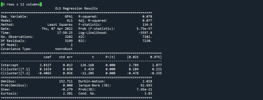

PLOT OUTPUT

ANALYSIS
3 adolescents in the cluster were considered for analysis:-
Cluster 0 - highest likelihood of having used alcohol
Cluster 1 - Most troubled adolescents
Cluster 2 - Least troubled adolescents
As a part of the analysis, it was observed that adolescents in cluster (the most troubled group) had the lowest GPA of 2.44; adolescents in cluster 2 (least troubled group, had the highest GPA of 3.01.
As a part of the tukey test, it was observed that the clusters differed significantly in mean GPA, although the difference between cluster 0 and cluster 2 were smaller.
0 notes
Last Seen Blogs

venomoftheshank
Ask Venomshank

kdrixx
Kyle Steve Foxx

kootical
𝐉𝐉 ֶָ֢⁷🍡
kootical
𝐉𝐉 ֶָ֢⁷🍡

majianguo
Explore, Teach, Travel