#juniper publishers indexing juniper publishers journals
Text
Hyperparathyroidism in Pregnant Women: Clinical Issues, Laboratory Findings and Relevant Therapeutic Approachesr - Juniper Publishers

Juniper Publishers- Open Access Journal of Annals of Reviews & Research
Hyperparathyroidism in Pregnant Women: Clinical Issues, Laboratory Findings and Relevant Therapeutic Approachesr - Juniper Publishers
Authored by Rosita Fontes
Abstract
Primary hyperparathyroidism (PHPT) is the most common cause of hypercalcemia in outpatient settings, with an incidence in women of reproductive age of 4.7-6.2 cases per 100,000 persons. When untreated in pregnant women, PHPT can lead to maternal and fetal complications. The authors present a case of a patient with a pre-pregnancy hyperparathyroidism diagnosis: she had worsening symptoms during pregnancy, so was referred for surgery due to failure of clinical treatment to keep the disease under control. Clinical issues, laboratory findings, and relevant therapeutic approaches are discussed.
Keywords: Hyperparathyroidism; Hypercalcemia; Multiple endocrine neoplasia syndrome; mTc-sestamibi scintigraphy; Beta chorionic gonadotropin; Parathyroidectomy; nephrolithiasis; calciuria
Abbreviations: PHPT: Primary Hyperparathyroidism; MEN: Multiple Endocrine Neoplasia Syndrome; BP: Blood Pressure; US: Ultrasound
Introduction
Primary hyperparathyroidism (PHPT) is a disorder that results from hypersecretion of parathyroid hormone (PTH), which is the most common cause of hypercalcemia in the outpatient setting. An analysis published in 2013 showed that the incidence in women of reproductive age, within a racially mixed population, is 4.7-6.2 cases per 100,000 persons [1]. In pregnant women, the disease occurs in 0.5-1.4%, and in 80% it is due to adenoma of the parathyroid glands [2]. When untreated, PHPT can lead to maternal complications such as nephrolithiasis, pancreatitis, and eclampsia, and fetal complications such as low birth weight and neonatal seizure [3-6]. Adequate control of patients who become pregnant with hyperparathyroidism can be a challenge, depending on their clinical symptoms and the laboratory and imaging evaluation. According to the trimester of pregnancy and severity of the disease, the treatment may be either clinical or surgical. The authors present a case of a patient with a pre-pregnancy diagnosis, and a worsening of symptoms during pregnancy; she was referred for surgery due to failure of clinical treatment to keep the disease under control.
Case Presentation
A pregnant 45-year-old woman, Afro-descendant, gravida 3, para 1, presented with a history of recurrent bilateral nephrolithiasis since she was 40 years old. She had a left wrist fracture after falling from height. Her past medical history was notable for low calcium intake, asthma and diabetes mellitus type 2, which was under control with metformin. In her surgical history, she underwent ureteral stent double J, and ectopic pregnancy surgery. She also suffered a lithotripsy for treatment of kidney stones. She presented for consultation for investigation of repetitive renal stones, denying any symptoms compatible with hyperparathyroidism. In her family history, there were no cases of hyperparathyroidism, no multiple endocrine neoplasia syndrome (MEN), or other syndromes associated with hypercalcemia. On physical examination, the patient was overweight (BMI 28.72 kg/m2), blood pressure (BP) was 110/75 mm Hg, bone deformities or fractures were not observed, and renal fist-percussion was negative. There were no other abnormalities found.
At admission, she brought examinations showing parathyroid hormone (PTH) of 390 pg/mL (12-65), total calcium corrected for albumin of 9.5 mg/dL (8.4-10.5), phosphorus of 2.3 mg/dL (2.5-4.5), as well as urinary calciuria in 24hours of 359 mg/day (100-250) and 4.78 mg/kg/day (< 4.0). Thyroid function tests were normal, as well as hemogram and biochemistry assessments. In several tests requested to confirm these results, her serum calcium was high (Table 1), along with maintained high PTH, low phosphate, and high calciuria. The parathyroid glands were not visualized on cervical ultrasound (US), but parathyroid 99mTcsestamibi scintigraphy (MIBI) showed hypercaptation of the tracer after 2 hours in the left lower parathyroid projection area, suggestive of a parathyroid adenoma (Figure 1). Renal US showed bilateral cortical stones, without lithiasis in the pyelocalyceal system. Adequate hydration and furosemide 20 mg/day were prescribed.
The 25-hydroxy vitamin D (VD) was low, 7.1 ng/mL (>30 ng/ mL), and the 1.25-dihydroxy vitamin D (1.25(OH)2D) was 193.9 pg/mL (18-78). She had recently presented with visual turbidity, nausea, headache, asthenia and dizziness, and recurrent renal colic, with an episode of pyelonephritis that was treated with antibiotic therapy. As the patient had a 2-week menstrual delay, a beta chorionic gonadotropin (beta-HCG) test was ordered, and the result was compatible with pregnancy. The gestational age calculated by the date of the last menstrual period was 5 weeks and 2 days. PTH and calcium remained elevated during the first trimester of pregnancy (Table 1). The option at that time, after discussion with the obstetrician, was increased furosemide at 40 mg/day and intensification of hydration. During the second trimester, the calcemia increased even more (Table 1), with the symptoms persisting. At that point, VD replacement was prescribed, and surgery was indicated. Parathyroidectomy was performed at 25 weeks of pregnancy, which was carried out without incident. On the first postoperative day, the patient had no symptoms, and the corrected calcium and PTH were normal (Table 1), although anatomopathological exam confirmed parathyroid adenoma. The pregnancy progressed without intercurrences. At 38 weeks and 2 days, she had an uneventful cesarean delivery. The newborn was healthy, with APGAR 9 at 1 minute and 10 at 5 minutes, 3.990 kg, and 49 cm, with no symptoms or laboratory evidence of hypocalcemia.
Discussion
PHPT is a rare condition in pregnancy [2,7].We present a PHPT case who became pregnant even with a diagnosis of the disease previously confirmed, and then underwent surgery for adequate hypercalcemia control. For the general population, hypercalcemia is defined as total serum calcium above 10.5 mg/ dL (>2.6 mmol/L). In a pregnant patient, the serum albumin falls due to hemodilution and remains low until delivery. Calcium is transferred through the placenta to mineralize the skeleton, and the glomerular filtration rate is increased, culminating with lower total calcium levels. Due to these factors, the upper limit of the reference range for corrected calcium in pregnancy is about 9.5 mg/ dL (2.3 mmol/L) [8,9]. This patient became pregnant at 45-yearsold. In addition to increased calcium and PTH, she presented with low phosphate and elevated 1.25(OH)2D. Most patients with PHPT are older than 50, but the disease is diagnosed during childbearing years in 25% of females [10]. Inappropriately high serum PTH concentration leads to increased renal reabsorption of calcium, phosphaturia, and 1.25(OH)2D synthesis, resulting in hypercalcemia and hypophosphatemia, loss of cortical bone, hypercalciuria, and various sequelae of chronic hypercalcemia [11]. During the course of her pregnancy, the patient presented symptoms of hypercalcemia as the serum calcium increased; such symptoms do not depend on gestational age, as they are the same for non-pregnant women [6,12].
A pregnancy in a patient with hyperparathyroidism may have maternal complications of 67%, and in neonates it would be about 80% [2]. The most frequent maternal complications are hyperemesis and nephrolithiasis; less frequently, preeclampsia and pancreatitis occur [2,6]. Fetal complications may include miscarriage, neonatal seizures, low birth weight for gestational age, and hypocalcemia [3,13]. This patient and her newborn did not present complications, probably because gestation was monitored from the beginning and surgery was performed in the second trimester to control calcemia. In a normal pregnancy, PTH levels are low during the first trimester compared to nonpregnant women and remain normal through the rest of the pregnancy. The relatively low PTH may be due to the suppressive effect of raised 1.25(OH)2D [14]. In this patient with primary hyperparathyroidism, high PTH levels were due to the autonomic secretion of the adenoma, preventing its fall as calcium levels raised. As such, continuous reabsorption of calcium of the bones occurs, as well as an increase of the tubular reabsorption of calcium, including intestinal absorption secondary to 1.25(OH)2D levels [15]. This modifies what physiologically occurs in gestation, when maternal calcium falls by about 10%; the current patient presented calcium within reference values at the beginning of the investigation, which increased progressively. The therapeutic measurements in the first trimester were sufficient to maintain serum calcium at the maximum level of 11.6 mg/dL (2.89 mmol/L); however, in the second trimester, calcium increased to 12.76 mg/dL (3.18 mmol/L). The incidence of pregnancy loss and its relationship to calcium elevation is not entirely known. Fetal loss is seen at all levels of elevated maternal calcium, but it is suggested that calcium levels higher than 11.4 mg/dL (2.85 mmol/L) may increase the risk of adverse events for both mother and fetus [16].
The patient urinary calcium was already high before pregnancy, with previous nephrolitiasis. Characteristic of the gestational period is an increase of calciuria [17]. Despite increased fluid intake, the risk of new kidney stones could be high, especially because she was put on furosemide in order to control hypercalcemia, which was an additional concern in deciding on surgery. This patient had low levels of VD. It has been demonstrated that even in tropical countries, its prevalence in pregnant women may exceed 80% [18,19]. In a normal pregnancy, 1.25(OH)2D may be twice as high compared to non-pregnant women [17]. However, this patient’s 1.25(OH)2D was very high: levels of the transporter 1.25(OH)2D protein, secondary to hyperestrogenism proper to gestation, and an increase in free 1.25(OH)2D production (due to increased activity of 1 alpha hydroxylase stimulated by parathyroid hormone-related protein (PTHrp), estrogen, prolactin, and placental lactogen hormone) are relevant factors that contribute to this issue. In addition, the synthesis of 1.25 (OH) D is increased by the activity of placentary 1 alpha VD hydroxylation [20,21]. In this case, elevated PTH was an additional factor that increased the 1.25(OH)2Dto such high levels. We prescribed VD based on the low levels presented, since the patient would need surgical correction of the hyperparathyroidism, with 1.25 (OH) D returning to normal pregnancy levels (and thereby revealing VD deficiency). There are no specific guidelines for treatment of hyperparathyroidism during pregnancy, as the approach is individualized according to the severity of hypercalcemia, the symptoms presented, a worsening of the clinical condition, and laboratory parameters.
During pregnancy hydration, enhancement and forced diuresis are measures that can avoid severe increases in serum calcium. The medications used for this purpose are class C and D for a pregnant woman, including calcitonin, cinacalcet, and furosemide. Bisphosphonates belong to category D [5,22]. We decided to prescribe a category C drug, with furosemide being the most accessible medication for the patient. However, a 40 mg/ day dose was not sufficient to control hypercalcemia, as she had continued clinical symptoms; thus, we decided not to introduce a new medication, but to refer the patient to surgery in the second trimester. Surgery is avoided in the first trimester due to increased risk of miscarriage, and in the third trimester, due to risk of preterm birth [23]. Although uneventful surgery has been done in the third trimester [24], the second trimester is the ideal time, as it is the period with potentially lower risks for fetal complications [12,25]. The patient underwent surgery, with excision of the left inferior parathyroid at the end of the second trimester: both she and the newborn were free of complications.
Conclusion
Patients with hyperparathyroidism who become pregnant need special attention for the development of clinical symptoms, the monitoring of laboratory parameters, and appropriate therapeutic interventions, given the occurrence of certain events. Since the management of pregnant women with hyperparathyroidism is relatively limited, we present a successful case here, which is aimed at discussing its clinical aspects, expected laboratory changes, and therapeutic possibilities.
To know more about Juniper Publishers please click on: https://juniperpublishers.com/aboutus.php
For more articles in Open Access Journal of Reviews & Research please click on: https://juniperpublishers.com/arr/index.php
To know more about Open Access Journals please click on: https://juniperpublishers.com/journals.php
#reviews research paper#Juniper Publisher Reviews#JuniperPublishers#Hyperparathyroidism#Multiple endocrine neoplasia syndrome#juniper publishers indexing juniper publishers journals
0 notes
Text
Palaeoenvironmental Background for the Early Paleolithic Occupation of the Volcanic Upland in the South Caucasus
Abstract
Nowadays, it has been reliably established that the Early Paleolithic people producing both Oldowan and Early Acheulian industries initially occupied the volcanic upland of the South Caucasus not later than 1.9.1.85Myr (Olduvai subchron). This period was characterized by a much lower relief than at present and subtropic climate that favored a dispersal of the early humans. The volcanic activity created there fertile paleosols with grass covers feeding hunted herbivores as well as rocks suitable for manufacturing lithic artifacts. In the subsequent periods of the Early and the Middle Pleistocene the upland underwent uplifting that led to a gradual deterioration of climate and appearance of glacial-interglacial rhythms with an increasingly pronounced difference between warm and cold periods. However, the chronological ranges of the studied Acheulian sites suggest that the humans continued to occupy the region under both more and less favorable conditions. The early humans are believed to have spread most widely in the region in the Late Acheulian, supposedly during in the Holstein interglacial.
Read More about this Article: https://juniperpublishers.com/ijesnr/IJESNR.MS.ID.556189.php
Read More Juniper Publishers Google Scholar: https://scholar.google.com/citations?view_op=view_citation&hl=en&user=4WXzQFMAAAAJ&citation_for_view=4WXzQFMAAAAJ:HoB7MX3m0LUC
#Juniper Publishers in USA#Juniper Publishers group#environmental science#sustainable development#Juniper Publishers PubMed Indexed Journals
0 notes
Text
Citrus Canker in Sudan: Etiology and Epidemiology- Juniper Publishers

Citrus bacterial canker disease (CBCD) caused by Xanthomonas citri subsp. citri (Xcc), is one of the most destructive diseases to the citrus plantations worldwide, newly invaded, and threatened citriculture in Sudan. Occurrence and spread of CBCD in Sudan have been surveyed in two states, representing the main citrus producing states in Sudan. Field surveys were conducted during January 2015 in commercial citrus orchards and nurseries at the two locations. Symptomatology, host range study, physiological and biochemical characterization of the isolated pathogen were also carried out to obtain important clues on pathogen identification. In addition, the pathogenicity test was performed on detached leaves of several selected citrus varieties such as grapefruit, orange and lime to establish the identity of the presumptive Xanthomonas citri subsp. citri (Xcc). The disease on lime orchards in northern and southern Sawagi (Kassala State) recorded a disease incidence of 66.6% and 18%, respectively. In nurseries, the disease incidence attained 51.7% and 53.6% in northern Sawagi and southern Sawagi, respectively, while in Khartoum State the disease was unexpectedly detected at a considerably high incidence of 45%, but at only one nursery, no disease detected in Khartoum State` s orchards during these surveys. Lime trees displayed typical symptoms of CBCD, but nearby canker-susceptible citrus species, such as grapefruit (C. paradisi) and sweet orange (C. sinensis) were unaffected. Typical symptoms of CBCD were noticed on leaves, twigs, fruits and branches. The pathogenicity tests of the recovered canker isolates induced typical lesions on local lime only, but produced atypical lesions on other citrus varieties. All the biochemical and physiological characteristics obtained from the re-isolations were also indicative of the presence of Xcc. As important perspectives, it appeared that these citrus canker isolates were distinctive and specific on lime. They were very similar to the pathotype and they attained an epidemic level in Kassala State.
Keywords: Citrus bacterial canker; Severity scale; Pathogenicity; Pathotype
Introduction
Citrus (Rutaceae family) is considered as one of the most important commercial fruit crops. Sudan, with all its vast area, wide range of soils, diverse climatic conditions, and ample water resource possesses great potentials for citrus production. At present, the commercial citrus production in Sudan spreads all over the country, mainly along the narrow strips of alluvial soils of the main River Nile, Blue Nile, and White Nile. In addition, it is also extending to the banks of annual valleys and rivers and upper terraces in which underground water is available for irrigation [1]. The important citrus groups have grown commercially in Sudan include: Small fruited acid lime (Citrus aurantifolia Swingle), grapefruit (C. paradise Macfad), sweet orange (C. cinensis Osbeck), and Mandarins (C. reticulate Blanco). Each group is composed of several varieties and selections (Ali-Dinar, 1984). The total area of citrus production in Sudan is estimated around 171,192 hectares with a total production of 2.3 million tons and exportation amounting to 9.8 thousand tons, for years (2010-2013) (National Horticulture Administration, 2013). Therefore, the national strategy of citrus expansion is directed towards the large national schemes, e.g. Gezira, Suki, Rahad and the Blue Nile Schemes in the Central Clay Plain [2]. Although the citrus crop is kept in great esteem, yet its present status is threatened by several problems, including low productivity caused by diseases. The citrus tree is attacked by several diseases in Sudan like gummosis, citrus decline, Tristeza virus, and virus-like diseases [3]. More recently a new aggressive disease was discovered in Gadaref State on lime with typical symptoms of citrus bacterial canker [4].
Citrus bacterial canker disease (CBCD) caused by Xanthomonas citri subsp. citri (Xcc) is probably one of the most devastative to the citrus plantations at the global level. Citrus canker is thought to have originated from South East Asia or India and spreading in more than 30 countries throughout the world, including countries in the Middle East, the Horn of Africa, and some other countries in South and West Africa [5,6]. Citrus canker disease is occurrence regularly on several citrus cultivars in varying degrees of incidence depending on the climatic conditions. The bacterium causes different symptoms ranging from pustules to necrotic lesions consisting of erumpent corky tissue surrounded by water soaked tissues and yellow halo on leaves, stems, and fruits [7-12]. As such, disease severity on susceptible variety results in defoliation, dieback, premature fruit drop, and blemished fruit, which consequently decrease fruit production and market value [13]. Also, the citrus canker has had a serious impact on local citrus industries whenever infections have been detected. As a result, millions of dollars are spent annually on prevention, quarantine, eradication programs, and chemical control [14]. Three main types of citrus canker bacteria have been identified, which possess variations in host range among citrus varieties.
The pathotype A (the Asiatic type of canker, Xcc) is the most destructive and widespread variant of the disease among most commercial citrus varieties and their relatives. The pathotypes B and C of citrus canker are caused by Xanthomonas fuscans subsp. Aurantifolii. Cancrosis B and cancrosis C are limited in host range and are geographically restricted to South America [15]. Certain distinctive groups within pathotype have also been identified which have restricted host range. For instance, pathotype strains with a host range restricted only to Mexican lime (Citrus aurantifolia) but not infecting citrus canker susceptible species, grapefruit and sweet orange, have been described in several countries in The Middle East and also reported from Thailand, Mali, Ethiopia, and Burkina Faso (Derso et al., 2009). Recently Elhassan et al., [4] reported the presence of CBCD for the first time on lime trees in Gadaref State (Sudan) depending on the visual symptoms, pathogenicity tests, and some biochemical characteristics of the causal bacterium isolate, which closely resemble the atypical Asiatic form of CBC . Now the disease seems to flare-up and spread to most of the citrus groves in Gadaref and Kassala states. It was also observed to spread in nurseries of Khartoum North. In general, the environmental conditions, particularly the climate are conducive to CBCD development in the remaining areas of all southeastern region of Sudan. Apparently, a high infection potential dominates the epidemiological stage in this region. The study was conducted to survey the natural occurrence, citrus varietal susceptibility, symptomatology, disease severity and extent of spread of citrus bacterial canker disease (CBCD) in commercial citrus orchards and nurseries in Kassala and Khartoum states, it was also aimed to confirm the identity of the causal pathogen depending on phenotypical characteristics and the pathogenicity of the bacterium isolates.
Material and Methods
Field survey and disease pathometry
The survey was carried out in January 2015 after the end of the rainy season in two different locations (Kassala and Khartoum states). In Kassala State, the survey was conducted in North Sawagi and South Sawagi areas, while in Khartoum State, the survey was conducted at Shambat in Khartoum North and at Almogran in Khartoum. The survey included inspection of two main citrus planting types namely, commercial orchards and nurseries. 6 orchards and nurseries per location at Kassala State and 4 from each were inspected at Khartoum State. Two hundred lime trees, in addition to 30-100 orange, mandarin, and grapefruit trees, whenever available, were examined in the same orchard inspected for the presence of CBCD. Also, all nursery stocks found at the selected sites were examined for CBCD. The main objectives of the survey were to discover the occurrence and extent of the spread of citrus bacterial canker disease (CBCD) and study its Symptomatology. Close visual observations were made and diseased plant tissues including, leaves, twigs, and fruits were collected from symptomatic plants. Disease development was then evaluated according to the following pathometry:
Disease incidence
The disease incidence (DI) was recorded for each planting type at these locations and the data were arranged and statistically analyzed. The calculations were based on the following formula:
DI (%) = No.of infected plants x 100 / total No. of plants inspected
Disease severity
i. In orchards
Ten trees were randomly selected at each orchard. Diagnostic symptoms were examined on leaves, fruits, twigs, branches, and the main tree stem. In severe cases, defoliation, twig dieback, and fruit drop were also considered. Disease severity (DS) was estimated at specified dates based on a 0-5 disease severity scale (SS) as the fallows:
Scale 0: non-symptomatic trees. Scale 1: leaf symptoms on few (1-3) branches, Scale 2: leaf symptoms in up to 10% of branches. Scale 3: leaf symptoms in >10%-25% of the branches plus mild symptoms on fruits and twigs. Scale 4: >25% -50% of the tree canopy showing clear canker symptoms on leaves, fruits, twigs, in addition to defoliation and die-back. Scale 5: > 50% of the tree canopy showing prominent canker symptoms on leaves, twigs, fruits, main branches, and trunks. Also, severe defoliation and dieback are evident.
ii. In nurseries
Disease severity was estimated based on a 0-5 disease severity scale (SS) as follow:
Scale 0: non-symptomatic nursery plants. Scale 1: leaf symptoms on few (1-3) leaves. Scale 2: leaf symptoms on 4 to 9 leaves Scale 3: leaf symptoms on 10 to 15 of the leaves. Scale 4: leaf symptoms>15 leaves to 50% of the foliage. Scale 5: > 50% of foliage showing canker symptoms. Besides, some individual lesions on twigs and stems are evident.
The disease severity (DS) was then calculated as follow:
3- Percent disease index (DX): It was calculated according to the fallowing formula:
DX (%) = DS x 100/ max SS
The recorded data on disease pathometry (disease incidence and disease index) were transformed using arcsine transformation, before being subjected to analysis of variance (ANOVA), as described by Gomez and Gomez (1984) for the factorial experiment in a completely randomized design. EXCEL computer package version 2010 was applied. Then the treatments means were compared using the least significant difference (LSD).
Symptomatology
Symptoms development of citrus bacterial canker infection was closely examined during the survey of the disease in each of chosen orchards and nurseries. Different parts of symptomatic trees were examined for canker lesions namely, leaves, twigs, fruits, branches, and stems. Also, leaf defoliation and die-back in twigs and branches were also observed, recorded, and photographed. The symptoms were closely noticed and described.
Isolation and purification of Xanthomonas axonopodis pv. citri
Isolation and purification of the bacteria from infected leaves, fruits, and twigs were conducted following the National Diagnostic Protocol for Asiatic Citrus Canker [16].
Pathogen identification
Morphological, biochemical and physiological characteristics of bacterium isolates including gram staining reaction, growth on YDC medium, starch hydrolysis, growth at 36 oC and 40 oC test, motility test, anaerobic growth, KOH Solubility test, (1-3%) NaCl Tolerance, gelatin liquefaction test, Tween 80 lipolysis and catalase test have been conducted according to Verniere et al [17], Goszczynska et al [18] and Kidist [19].
Pathogenicity Test
Pure isolates of the bacterium were grown on nutrient agar plates and incubated at 28℃ for 24 h. Bacterial cells were then harvested in sterile distilled water by using a sterile glass rod and the bacterial suspension was adjusted finally to give 1.0 × 10⁸ CFU/mL using a UV spectrophotometer at a wavelength of 600 nm (Sunrise Spectrophotometer, Tecan). Immature fully expanded ‘Mexican’ lime and ‘Marsh’ grapefruit, Valencia orange, Eureka and Mandarin leaves were sterilized by soaking for 2 min in 1% sodium hypochloritae followed by rinsing in sterile distilled water. Leaves were placed on the surface of 1% water agar with their abaxial surfaces facing upwards. Six wounds were made per leaf with a needle and droplets (10 microliters) of bacterial suspensions were placed on each wound. Leaves were incubated at 280C with a photoperiod of 12 h light and 12 h dark for 2 weeks.
Results
Field survey and disease pathometry
The survey conducted in commercial citrus orchards and nurseries in both Kassala and Khartoum States indicated the occurrence of citrus bacterial canker (CBC) on lime (Citrus aurantifolia Swingle), but not on the other surveyed citrus varieties. While the typical disease symptoms in Kassala State were evident in both citrus orchards and the nursery lime seedlings, they were only displayed in the nursery stock and absent in orchards in Khartoum State. The combined disease development of the two planting types (orchards and nurseries) in Kassala State was consistently significantly (P ≤ 0.05) higher in Sawagi North compared to that in Sawagi South (Table 1). Separately, CBC development on each planting types was as follows:
i. In orchards
The results of the disease Incidence, severity, and disease index are shown in Table 1. The disease was recorded in all surveyed commercial orchards in Kassala State. While Sawagi North recorded significantly (P ≤ 0.05) higher CBC incidence (66.6%) comparatively low disease level was recorded in Sawagi South (18%). Similarly, more severe CBC (3 fold as much) was encountered in Sawagi North with a disease index, which was significantly (P ≤ 0.05) higher (64.9%) than that recorded in Sawagi South (25.3%). However, the disease was not detected in citrus orchards in Khartoum State.
ii. In nurseries
Citrus bacterial canker disease was recorded in all the surveyed nurseries in both locations of Kassala State (Table 1). North Sawagi recorded 51.7%, 2.1 and 52% CBC incidence, severity, and disease index, respectively. Comparable CBC development was noticed in South Sawagi indicating 53%, 1.8 and 51.5% incidence, severity, and disease index respectively. However, In Khartoum State, the disease was detected in 45% of lime plants in only one nursery in Khartoum North with an overall mean disease incidence of 12.6%, moreover, 0.7 and 21.2% CBC severity and disease index were recorded respectively.
Symptomatology
Typical symptoms were observed upon examination of 'local' lime trees infected with CBC (Figure 1). These characteristic external symptoms were cankerous pustules and necrotic lesions consisting of raised or erumpent corky tissues on leaves, fruits, twigs, thorns, and branches. The canker lesions on leaves and fruits were surrounded by a water-soaked ring and often with a prominent yellow margin. Also, lesions with a shot hole-like appearance were found. Unusual canker lesions were also commonly encountered on the leaves, which were associated with mechanical (i.e. thorn) and leaf miner damages. Many of these canker lesions coalesced to form elongate or blotchy corky patterns on the affected leaves. Frequently, severe infections were encountered in some surveyed orchards which largely covering. In severe cases of foliage infection, extensive leaf defoliation and die-back symptoms were observed. The fruits were particularly susceptible to the canker pathogen, usually developing severe canker lesions with crater-like centers and severe gummy exudates. Which ultimately led to piles of fallen fruits underneath the affected lime trees. In nurseries, severe canker symptoms were also observed on leaves, twigs, and stems (Table 2).
Pathogenicity test on detached leaves:
The typical canker lesions observed on infected lime leaves were reproduced only on lime in response to the pathogenicity test performed on detached leaves. On day 7 post-inoculation small white callus developed on lime leaves at the six inoculation points (Plate 12A). Advanced callus formation gradually changing to tan color lesions surrounded by water-soaked area and yellow halo were produced on lime leaves as time progressed to 20 days after inoculation (Plate 13A). A typical symptom of flat lesions developed on sour orange, ʻValenciaʼ orange, and ʻBaladiʼ mandarin (Plates 13B, 14A, 14B). However, ʻEurekaʼ lemon, ʻMerkisʼ mandarin, and grapefruit (Red blush and March) failed to produce any symptoms (Plates 15 and 16) similar to the control treatment inoculated with sterile distilled water (Figure 2).
Discussion
The citrus bacterial canker disease (CBCD) has become established and attained an epidemic status in different parts of Sudan. Although the disease has not been known before 2013, its emergence in autumn 2014 was somewhat overwhelming and so intriguing. It infested the main citrus growing areas of Kassala State which represents the most important commercial producing region in the country, particularly the North Sawagi and the South Sawagi localities recording considerably high CBCD levels (incidence of 66.6% and 18% and disease indexes of 64.9% and 25.3%, respectively). This outbreak is believed to have been caused through a long-distance spread, which more often occurs with the movement of infected propagating materials such as nursery stocks, budwood or budded trees, or through contaminated environmental factors such as nursery workers carrying the bacteria on hands, clothes, and contaminated budding tools [11]. Alternatively, the spread of canker bacteria may have occurred during strong wind-driven rains coming from Gadaref State or across the borders from Ethiopia (Derso et al., 2009) or Saudi Arabia [6]. The fact that CBCD was first detected in some Gadaref State localities only a year before it appeared in Kassala, would indicate that the path of the disease was most likely: Ethiopia- Gadaref then Kassala. This could be substantiated by the discovery of the disease several years ago in Ethiopia (Derso et al., 2009) and only recently in commercial citrus orchards and nurseries of Gadaref State [20]. The bacterial inoculum might have been present in Kassala in the same year of the discovery of CBCD in Gadaref, but it has been overlooked since the pathogen is known to survive epiphytically at low population levels on citrus hosts without symptoms development, and in association with other weeds and grass hosts [21,22]. However, the bacteria survive primarily in naturally occurring lesions. Cankerous leaves, twigs, and branches constitute the main source of the inoculum, but the prominent occurrence of lesions is seasonal, coinciding with periods of heavy rainfall, moderate temperature, and growth flushes. The pathogen can survive up to 6 months or more in the infected leaves [23] and up to 76 months on diseased twigs [24].
In comparison, the greater CBCD development in the Northern Sawagi over that in the Southern Sawagi can be attributed mainly to the topographical factors of Kassala State heights (≤ 850 m a.s.l). These heights may retard the wind speed in South Sawagi, while in North Sawagi orchards on the other side exposed to wind-driven that may carry the bacterial inoculum. Also, the variation of disease pathometry may have a direct relation to differences in the prevailing cropping systems in the two locations. For instance, the mixed plantation of lime /mango system makes southern Sawagi trees less infected because of the windbreak effect created by mango trees. This is not surprising since cankers develop more severely on the side of the tree exposed to wind-driven rain. [25]. Although this variation in CBCD level is perceivable in the first year of the appearance of the disease, it is unlikely to persist if the locally prevailing epidemiological factors remain remarkably similar in the two locations.
On the other hand, CBCD was absent in Khartoum State, be it in commercial citrus orchards or nurseries, except in one nursery of lime seedlings in Khartoum North. This was perceivable since the prevailing environmental conditions were not conducive for CBCD development [26]. The remarkably high CBCD incidence reported in that nursery (45%), however, was believed to have resulted from a consignment of infected nursery stock brought from infested wet areas such as Kassala or Gadaref. It may constitute a potential threat, at least in localized small pockets in Khartoum State where the temperature and humidity may allow for a limited occurrence and spread of the disease. The study also demonstrated that the epidemic was naturally occurring and spreading on acid lime trees (Citrus aurantifolia) but not on other citrus varieties, even if they were close to the diseased lime trees. This strongly indicates that this citrus canker bacterial isolate is restricted to lime. The host specificity of this canker bacterium to lime was like that from Gadaref [20], which would further support the notion that it originated from Gadaref. The canker bacterium isolates which are specific to lime have also been previously reported from Maldive islands [26], Southwest Asia [5], Ethiopia (Derso et al., 2009), and the western region of Saudi Arabia [6]. The fact that the pathogenicity tests of the isolated bacterium developed characteristic lesions only upon artificial inoculation of detached leaves of lime and failed to induce any cankerous lesions typical of citrus bacterial canker (CBC) on grapefruit, sweet orange, or on other citrus varieties tested was a strong indication that the present bacterial isolate may belong to a special group of strains designated as pathotype A*. Although closely related to the ordinary A pathotype, these strains can be readily distinguished from the former, based on their atypical combination of host range and symptomatology [5]. Additional strains with similar biological behavior were reported by [7] and were also included in this distinctive group (i.e. A*). Although this bioassay has been found in both specific and sensitive diagnostic methods for CBC [8] the molecular analysis will certainly establish the correct identity of the bacterial isolates spreading in Kassala and elsewhere in Sudan. Collectively, the association and isolation of Xanthomonas sp. from symptomatic lime trees, together with the symptomatology, biochemical characterization, and pathogenicity tests strongly indicate that the currently investigated disease on lime in Kassala and Khartoum states is CBC (X. citri subsp. citri) and these lime isolates are closely related to the strains of the atypical Asiatic pathotype (Xcc- A*) [27-32].
To know more about
Journal of Agriculture Research-https://juniperpublishers.com/artoaj/index.php
To know more about open access journal publishers click on Juniper publishers
1 note
·
View note
Text
New Records of Sea Level Changes in the Fiji Islands- Juniper Publishers
Abstract
New sea level records from the Yasawa Islands in Fiji are presented. Beachrock occurs frequently on the beaches in the zone between mean and high tide levels on most of the islands. They date to the last 4200 years. The present sea level has produced distinct shore marks in the form of under-cut notches, rock-cut platforms and sea-caves in the bedrock, as well as sand accumulations with a clear mean high tide level (HTL). The fieldwork was concentrated in 10 sites. Elevation was measured with a high-precision instrument with respect to HTL. Ages were determined by 17 C14-dates. A +70cm higher sea level was observed, sampled and dated at AD 1530-1673. It was followed by a significant regression of about 1.7-1.8m, killing coral reefs and cutting a new rock-cut platform some 20-30cm above present mean low tide level (LTL). Then sea level rose again to its present position, or slightly above, a level, which remained fairly constant over the last 150200 years. In the last 60 years corals were killed due to a sea level lowering or a severe bleaching episode. After that very stable sea level conditions must have prevailed for the last decades, forcing corals at several sites to grow laterally into microatolls.
Keywords: Relative sea level changes; Regional eustasy; Rotational eustasy; Yasawa Islands; Fiji
Go to
Introduction
Before addressing our research project, it seems appropriate to review the regional background with respect to plate tectonics, regional geography, the interaction of changes in land and sea levels, and especially previous research achievements in Fiji with respect to sea level changes. It seems surprising to note that all previous work has been addressed to interglacial and Holocene sea level change older than the last millennium, because it is the sea level of the last 500-1000 years that have the potential to act as a key to our understanding of what is actually going in present time.
Plate tectonic setting
Fiji is positioned between plates of complex geodynamic force and motion (Figure 1). According to the Fijian Ministry of Land and Mineral Resources [1], the Lau-Colville Ridge and Fiji represent an old dormant island arc ridge (Figure 2). However, this area is still seismically active [2-4]. For example, Suva experienced a M 6.8 earthquake in 1953 and a M 7.1 earthquake in 2009. In the Yasawa Islands area, the subject of this paper, a M 6.8 earthquake occurred in 1902 and a M 6.1 earthquake in 1984 [2].
Geography of the Fiji Islands
The nation of Fiji consists of about 330 separate islands (Figure 3). The main island is Viti Levu with Vanua Levu the second largest. The sea level changes and archaeology of Viti Levu have been studied by [5,6]. The eastern island group known as the Vanuabalavu Islands have been investigated by [7]. Kadavu Island has been studied by [8]. The Yasawa Islands were the target of our own investigations with respect to sea level changes. The Mamanuca Islands have been studied by [9,10].
Changes in land and sea levels
The tide-gauges at Lautoka and Suva on Viti Levu (Figure 3) provide records of the relative sea level changes since 1992 and 1972, respectively. In the vicinity of the tide-gauge stations there are GPS stations measuring the changes in crustal level. Both tide-gauge stations seem very unfortunately placed on heavy harbour constructions resting on soft marine sediments susceptible to significant compaction, and can hardly be used to decipher the present trend of sea level changes [11].
Several authors have tried to apply a seismotectonic zonation of the Fiji Islands (e.g. [12-16]). According to [16] only the Ovalau-Moturiki Islands (just east of Viti Levu) represent stable tectonic conditions, however.
Previous sea level research
As far as we know, there have been no studies of sea level changes conducted in the Yasawa Islands, except for a few notes (e.g. [14]). In this case our investigation brings forward new material. On Viti Levu, the Ovalau-Moturiki Islands, the Vanuabalavu Islands, the Karavu Island and the Mamanucas Islands, there are previous investigations to consider. Before addressing those papers, there are a few general problems to consider.
Radiocarbon dates of marine material need to be calibrated with the so-called reservoir effect satisfactorily well determined. Petchey et al. [17] reports the ages of four modern shell and coral samples. The reservoir ages were around 450 years, a value we adopted and used as 450±30 years in our marine radiocarbon calibration via OxCalv4.2.4 [18]. This makes direct comparisons complicated as, for example, [5] used a reservoir value of 370 years and an old calibration curve [19], and [7] used 438 years and an older calibration technique [20].
The use of datum level is another subject of great difference. Both [5,7] use the lowest astronomical tide (LAT) as their zero- level. This is quite surprising as this level is a theoretic level [21,22] not recognizable in the field. The unfortunate choice of LAT as their zero-level generates problems with respect to the identification of past sea level index points.
Past sea level data can only be referred to MSL (usually more or less arbitrary, however), HTL (morphological features like notches, sea caves, rock-cut platforms and some beach structures) or LTL (microatolls). This implies that sea level graphs with a datum set at LAT become misleading as they show data points above the chosen LAT-datum, which in fact may not represent any higher sea level position.
It seems natural that the nautical charts are referenced to the low-tide level. But geological and biological associations to shore structures, corals in situ or marine shells and corals in shore deposits are all much better related to the high-tide level, which in most cases is very easily identifiable. Therefore the HTL was selected as the ideal datum. The mean-tide level is usually also easy to identify on a beach, as a minor break in slope and concentration of larger particles like coarse sand and gravel [23].
The present tidal range is given as 1.30m by NOAA [21] and maximum 1.84 for Suva and 1.82 for Nadi according to [24]. In the field, a tidal range of 1.51m was measured. The conversion to LAT is not obvious (and we have no information of what value previous authors have used), but it seems that LTL should be about +30cm, MTL about +100cm and HTL about +170cm with respect to the LAT-datum [25].
Finally, it is interesting to note that all the previous papers are devoted to Mid and Late Holocene sea level data, and that there is a general lack of data for the last millennium. This is why the study, being focused on the last 500-600 years' field evidence on sea level changes, will fill a gap in the sea level history of the Fiji Islands [26-27].
Viti Levu: Nunn & Peltier [16] listed 32 C14-dated samples from 11 sites on Viti Levu. Additional dates come from [9,28,29], and our dates from Maui Bay (below). The data are plotted in Figure 4.
From Rove Peninsula (SW Viti Levu), [28,29] have reposted a stratigraphical record spanning the entire Holocene. At around 8000cal.yrs BP marine influence is recorded at the -3m (MSL) level. At 8000 BP, global eustatic sea level was at about -10m [30], suggesting that the Rove Peninsula has been uplifted by about 7m since 8000 BP; i.e. at a mean rate of 0.875mm/yr. Therefore, there are good reasons to dismiss their maximum sea level of about +2.1m dated 4055±575cal.yrs BP (suggesting a mean uplift of 0.525mm/yr).
From Vuda Point, between Nadi & Lautoka, [9] describes microatolls of Porites sp. at 16cm below MTL dated at 6460±70 and 6350±60cal.yrs BP, which corresponds to a sea level position at about +0.8-1.0m. If eustatic sea level at that time was at about -2.0m, the Vuda Point area is likely to have gone up by 2.0m; i.e., at a mean rate of 0.312mm/yr.
Bloom [31] reports the finding of a submarine peat-bed in a drowned valley tributary to the Rewa River east of Suva dated at a depth of -4.5m with a C14-age of 5500±110 BP, corresponding to 6295±111cal.yrs BP. If we assume a eustatic position at that time of about -1.5m, the site would have gone down by 3.0m or at a mean rate of 0.476mm/yr, which seems reasonable for a delta area. Wood at -0.2m in the Rewa River delta has been dated at 4165±245cal.yrs BP. Even this date is likely to represent subsidence, and has therefore been ignored in the sea level graph of Figure 4.
Obviously, there must be differential tectonics involved; uplift of Rove Point, uplift of Vuda Point and subsidence of the Rewa River delta. All the other sites seem to provide a reasonably congruent picture (i.e. stability); viz. sea level at about +0.3m from 5600 to 4900cal.yrs BP, at about±0.0m 4150-3950cal.yrs BP, at about +0.3m around 3350cal.yrs BP and at about -0.5m from 2900 to 1500cal.yrs BP (as illustrated in Figure 4).
Ash [5] investigated three sites along the northeast coast of Viti Levu and had 7 samples radiocarbon dated. He concluded that sea level rose to about +0.45m by 5300 BP and "has since declined at a constant rate". He also claimed: "sea level has not been significantly raised since 1630±250 years BP". The last statement is seriously contradicted by the present findings in the Yasawa Islands, however (below).
The earliest inhabitants of the Fiji Islands were the Lapita people. Kumar et al. [6] reported the finding of charcoal dated at 2583±233cal. BP. Nunn [32] gives an age of the Lapita settlement of "approximately 1350-750BC" (i.e., 3300-2700BP). This is in good agreement with the general Lapita immigration according to [33] and the stratigraphic records from Tavua Island, west of Nadi, by [10].
We investigated a section at Maui Bay on the south-coast including a piece of pottery and shells dated at 4019±103cal. yrs BP (below), suggesting that people might have been present significantly earlier, however
The Ovalau-Moturiki Islands: The Ovalau Island lies just east of Vitu Levi with Moturiki Island close by. They were studied by [34]. According to [34] the islands "have been subsiding very slowly for most of the past few thousand years". According to [16], however, these islands represent stable tectonic conditions, and would hence record regional eustatic changes in sea level.
There are 10 C 14-dates from Ovalau Island and 7 from Moturiki Island [16]. When plotted against time, the data suggest that sea level was at around +0.5m (MSL) in the period 6500-4500cal.yrs BP and at about +0.4 to +0.7m (MSL) in the period 3500-2900cal.yrs BP. Two dates from +1.6m (LAT) of about 5700cal.yrs BP and from +1.5m (LAT) of about 3700cal. yrs BP are problematic [34].
The Vanuabalavu Islands: Nunn et al. [7] undertook an extensive survey of past Holocene and Pleistocene sea levels as recorded by shore notches and marine deposits. The story is backed up by 4 C 14-dates of Holocene deposits (below recalibrated according to the methods used) and 3 Th/U-dates of Last Interglacial material. As mentioned before, they use a theoretical LAT as their zero-datum, which poses problems with respect to the identification of morphological sea level criteria, according to [7] here "typically marked by shore platforms, notches, marine caves and, less commonly, fossil corals and beach deposits". In the text they often talk about elevation with respect to "its modern analogue" (which is to be recommended) and some drawings give elevation with respect to mean sea level (which implies a new zero level about 70cm above LAT).
Nunn et al. [7] observed 3 different shorelines in the Vanuabalavu Islands; an upper +9-10m level of unknown Pleistocene age, a +5m Last Interglacial Level, and a +1-2m Holocene level. Their records have been combined into a shoreline diagram in Figure 5, and supplied with some additional information. The Last Interglacial level (red) seems to go through all sites at a fairly uniform level of about +5m above MTL. The Holocene level (blue) is by no means uniform, varying between around +1m and +2m. Because of the uniform Last Interglacial level, the Holocene irregularities cannot be interpreted in terms of differential tectonics, but have to be from field interpretation; the +2-3m levels on Mago Island are far from clear, on Kaibu Island there are no such levels recorded, on Yacata Island the +2-3m levels are unclear, and this is also the case with the +2m level of Vatuvara Island. Much better and more conclusive are the +1m levels of Vanuabalavu and Namalata Islands. The data presented suggest an elevation of +0.9m to +1.3m and an age of 3540±170cal.yrs BP to 3959±180cal. BP (overlapping at 3745±69 years). Therefore, a +1.1±0.2m level with an age of about 3750cal.yrs. BP is proposed. The microatoll (Porites) at +0.2m on Avea Island is indicative of sea level stability around 4178±180cal.yrs BP at about +0.6m.
On the south tip of the Vanuabalavu Island, there is a big cave named the Qaranilaca Cave. Its floor is given as "approximately 2.1-2.5m above mean low-water spring tide" [35]. This datum is not very useful, but corresponds to 0.8-1.2m above HTL and 1.5-1.8m above MTL. The stratigraphy is interesting [7,35,36]. The top 70cm is a bed indicating human habitation. According to Nunn et al. [7], it represents a significant regression at about 300BP (AD 1788±114cal. yrs). Then follows a 7cm marine bed (with sharp boundaries below and above) at +0.25-0.30cm above HTL. Below that are two beds with human habitation material dated at AD cal. 660 to 1160. At the base, 50cm below HTL and 10cm above MTL, there is a second marine bed of sand and beachrock.
Kadavu Island: Nunn & Omura [8] studied the Quaternary sea level changes on Kadavu Island. Their tectonic interpretation seems hardly tenable. The structural observations, on the other hand, seem quite straightforward; a "reef limestone" reaching +7.1m and dated to the Penultima Interglacial around 210Ka BP (3 Th/U-dates given), an undated "predominant erosional bench" at +2.6-3.4m of assumed Last Interglacial age, and an absence of emerged Holocene levels. This is illustrated in Figure 6.
There is a clear difference in elevation of the three shorelines in Figure 4 (Vanuabalavu) and Figure 6 (Kadavu): The Penultima Interglacial level of +7.5-8.0m on Kadavu seems to correspond to the +9-10m shoreline (green) on Vanuabalavu, The Last Interglacial level at +3m corresponds to the +5m level in Vanuabalavu (red), and the absence of emerged Holocene levels on Kadavu correspond to the +1m level in Vanabalavu (blue). A Penultima Interglacial sea level at +7.5m calls for some tectonic uplift. At the same time, however, the Last Interglacial and Holocene sea levels are indicative of predominant stability. Therefore, it seems to represent an episodic uplift of at least 5m in pre-Last Interglacial time.
Mamanucas Islands: Morrison et al. [10], studied nine cay islands of the Mamanucas Islands, located between Vita Levu and the Yasawa Islands. Cay islands are small sandy islands of low elevation formed on top of coral reefs by the erosional debris of corals, mixed with other marine organisms. They reported C14-ages from 3 cay sand islands. The subsurface ages go back to about 2200cal.yrs BP. All the surface dates belong to the last 600 years. The study has little to contribute to sea level changes. It just supports the notion that sea level had changed from a general rise to a general stability (or fall as proposed by [16]) well before 2200BP.
Morrison et al. [10] studied Tuvua Island in the same island group with respect to sediment stratigraphy and archaeological material. Coral fragments without morphological relation to any beach structure were dated; one at +1.9m (MSL) at 2816±20BP and one at 1.75(MSL) at 3294±21BP, suggesting that sea level was at about the present level, or even somewhat higher. The archaeological remains have ages in full agreement with the age of Lapita immigration according to [32].
Methods
Before going to Fiji, we carefully scanned suitable coastal segments of the Yasawa Islands as recorded on Google Earth images. After that we selected our spots and formulated our fieldwork program. Sometimes, this was not easy because we were not sure how to arrange local transport. In the field, we investigated the morphological characteristics and decided about how to work with respect to levelling, photo documentation and sampling for C14-dating.
We used the mean high-tide level (HTL) as our datum because it was morphologically easily identified. This level is about 70cm above mean-tide level (MTL) or mean sea level (MSL), and about 170m above the lowest astronomical tidal level (LAT). Levelling was performed with a high-precision Kern instrument, implying a measurement accuracy of better than 1.0cm. Microatolls were observed and their upper top surface was measured with respect to the sea level at low tide to the minute of its lowest position. The photo documentation includes several hundreds of images taken by different cameras, including one under-water camera.
Radiocarbon AMS dates were performed by Professor Goran Possnert at the Ångström Laboratory at Uppsala University. The marine calibration was done according to OxCal v4.2.4, with a reservoir effect of 450±30 years applied [36].
Results from Fiji Island
Because the Fiji Islands were going to be the center piece at the UN conference in June 2017 [37] and at the COP23 conference in Bonn in November 2017 [38], there suddenly became an urgent need of a careful sea level investigation in Fiji with respect to present trends and recent to sub-recent changes in sea level. Therefore, we initiated a new sea level project in the Fiji [26]. After studies of coastal segments on Google Earth, we selected the Yasawa Islands as our main target.
Our field studies spanned 3 weeks in March 2017. The locations of our investigation sites are shown in Figure 7, and include four sites on Viti Levu (coastal observations at Denarau west of Nadi and at Maui Bay east of Sigatoka, and the locations of the tide-gauge stations Lautoka and Suva). However, our main investigation concentrated on 10 sites in the Yasawa Islands.
Studies on Viti Levu
The investigations on Viti Levu will be described as shorter notes under this section. The main report on our results from the Yasawa Islands will follow below.
The Lautoka and Suva tide-gauge stations
The study of the two tide-gauge stations at Lautoka and Suva has already been reported on [11]. Our main conclusion was: "Any application of mean trends would produce meaningless values rather misguiding than assisting in the handling of estimation of on-going absolute sea level changes".
This is important, and implies that we must seek other means of establishing the present trend in regional ocean level changes. Consequently, this was our main target in our fieldwork in the Yasawa Islands, besides recording sub-recent to Late Holocene sea level changes.
The Denerau Site
Our first contact with the shores of the Fiji Islands occurred at Denarau. The first observation was that there are absolutely no indications of the shore advancing inland due to sea level rise, on the contrary sea level seems to remain quite stable (Figure 8).
A second observation was that there was an upper limit of dead Patella shells, and a lower limit of living Patella shells (Figure 9). The difference in elevation is 10-20cm, and may suggest that there has been a lowering of sea level in sub-recent time.
The Maui Bay site
At Maui Bay Public Park, on the south coast some 21km east of Sigatoka, the accidental find of an interesting site of past sea level changes led to some important discoveries. There is a thick beachrock deposit outcropping in the intertidal zone of the present beach. Also, there is clear evidence of a somewhat higher sea level. In an erosional depression of a small brook, we found a stratigraphic section, documented in Figure 10. Three generations of shore deposits can be distinguished.
An extensive beachrock deposit has its surface planed into a rock-cut platform (RCP). The high water level was found in direct association only 5cm higher (HTL). The present beach sand deposition, unit III, goes up 110cm above HTL (zero in Figure 10). An older over-grown sand unit (II) goes up 90cm above the top of unit I, indicating that sea level at one time must have been higher than today by about 90cm or a bit less.
Underneath these sand units, there is a third unit (I). It has a 30cm-deep soil at its top, indicating considerable age. A piece of pottery was found at a depth of 10cm (sample 20 in Figure 10), indicating that the soil and sand unit has to be of Late Holocene age. Shells and corals at a depth of 20cm (sample 19) were C14- dated at 4244±26 BP, or 4345±100cal.yrs. BP. A 10cm thick bed of flint-hard beachrock occurs close by. Corals from this bed (sample 17) were C14 dated at 4005±26 BP, or 4019±103cal.yrs. BP. This means that shore unit I has an age of about 4182cal. yrs BP (the mean of the two samples). Obviously, sea level had reached the present level, but hardly above this level (at least not more than 0.5m).
A sea level at about ±0.0m at about 4200 BP is in minor contrast to the results of [5], who has a Holocene sea level maximum at +0.45m at 5300cal.yrs BP. Ash and Ash [39] demonstrated that a proposed +1.6m Holocene maximum [40], in fact, was only at a +0.48m level (MTL). A sea level at about +0.4-0.5m would agree with all three records, however, but strongly contradict a +2m level as suggested by [16].
The piece of pottery found in the soil (sample 20) with a date of 4019±105cal.yrs. BP implies that Lapita people are likely to have already arrived on Fiji by 4000 BP. As this is earlier than considered before (e.g. [10,33,35], it seems necessary to show the piece of pottery (Figure 11).
Results from the Yasawa Islands
The Yasawa Islands is a chain of six main islands and numerous smaller islets spanning 80km in a SW-NE direction (Figure 12). The islands were not charted until 1840. All islands consist of volcanic bedrock (Figure 13). Erosional products generate coastal sand beaches. We undertook detailed sea level studies in 10 separate places. In addition, we made important observations of the coast from the ferryboat as well as the small boats we used for local transportation. As part of our planning for this investigation, we studied all of the islands on Google Earth images.
At Viwa Island 25km to the west of the main Yasawa Islands, three coral samples have been Th/U-dated at the Last Interglacial [8], viz. 126±7ka BP from +2.1m, 128.7±1.6ka BP from 2.85m, and 136±12ka BP from +3.1m. According to [14] "no relatively emerged features of certain Holocene age are known from the Yasawa and Mamanuca Islands". This statement seems valid even today (except for the +70cm level described below).
The present shore forms a distinct line all around the islands of rock-notches, sea-caves and rock-cut platforms, as well as sandy beaches (Figure 14). These morphological elements are closely tied to mean HTL, and therefore constitute an ideal datum for our investigations. Levelling was undertaken with a high-precision Kern instrument with rod-readings of up to 0.51.0cm accuracy.
General coastal observations
All the way from Kuata Island in the south to Bukama Village in the north, we observed very distinct shore morphological elements indicating the HTL; i.e., bedrock notches, under-cut notches, rock-cut platforms, and sandy shore HTL marks.
A few examples of the distinct high-tide shore markers are given in Figure 15a-c. At some coastal segments it seems evident that the coastal sand is also graded to a somewhat higher level (+1m or less), now overgrown and not reached by the waves at the present sea level. This seems to indicate that there was, in sub-recent time, a higher sea level on the order of +0.5 to +1.0m (Figure 16a-b).
There seems to be a general lack of higher shore marks, either from a Late Holocene sea level maximum (as proposed by [16]) or from a Last Interglacial level (as found on Viwa Island to the west).
Bukama Village
We spotted the coast at Bukama Village on the Google Earth images and were attracted by sandy beaches disappearing against rock cliffs and a tombolo spit (Figure 17), both structures of which had a potential for recording changes in present sea level. We accessed the site via a 25km long boat ride from Nabua lodge. This ride provided excellent coastal views of distinct shore morphological features indicating the HTL (under-cut notches and sea caves) and sand beaches with the present HTL clearly visible and an older, overgrown, higher surface from a somewhat higher sea level at about +0.5-1.0m.
An extensive beachrock at point 1 (Figure 18) was C14-dated at AD 611±82cal.yrs. This implies that sea level at that time was at about the same level as today. Judging from the Qaranilaca Cave section on Vanuabalavu Island (section 1.4.2, above), this level was followed by a lower level lasting from about AD 660 to 1160 [35].
The tombolo spit is built out between the mainland and a small island (Figure 17). Figure 19 gives a view from the bedrock hill seawards. The tombolo is built out from the north to the south by converging long-shore drift. The crest, the washing (swash) limit (WL), and the HTL on both sides were leveled with our high-precision instrument (Figure 19 & 20). The vegetated part is no longer reached by normal waves, and was partly formed at a somewhat higher sea level. The crest is successively falling off to the south and there is a total lack of any signs of present rise in sea level, on the contrary stability is evident. At the foot of the rock hill, there is an old, inactive under-cut notch, now filled by sand (Figure 21a). It must have been cut at a former sea level somewhat higher than today. The leveling indicates that the former sea level must have been about 70cm higher than today (Figure 20). Besides the +70cm notch, there are erosional marks in the bedrock at +2.4-2.6m and at +5.5m (Figure 21b). Those marks perhaps represent former sea level notches. We are not sure how to classify them, and leave the question open by assigning them "possible higher sea level notches". No other site with higher notches was observed between Naisisili and Bukama (Figure 22). At Naisisili, there might be one (Figure 31).
Nabua Lodge and Naisisili Village
This site was selected because the Google Earth image showed a long coastalspur (Figure 23), which by precise leveling might provide insight into the present trend of sea level; whether rising, stable or falling. Naisisili Village lies on a sandy flat between the sea and a small brook running parallel to the shore for about 600m. Today, the area of the village is not reached by the normal waves. The sandy ground of the village represents littoral swash deposits at a former sea level in the order of 0.5- 1. 0m higher than today's sea level. The shore spur to the south is graded to a lower level. The situation is illustrated in Figure 24.
The shore spur (spit) was subjected to precise levelling with 7 sections crossing the spit, identifying the present HTL, the sand/vegetation limit, the crest on the seaside, and the lagoonal HTL both the inner side and the foot of the back-side escarpments (Figure 26).
Figure 26 gives the main levels identified along and across the shore spur. The crest falls off from around +2m in the north to +1.5m in the south. The shore spur is 155m long. A C14-date of shells 30cm below surface gave an age of 532±23BP, which in calendar years is AD cal. 1866±82. Assuming an age of about 150 years for the spur to form, it would have been built out to the south at a speed of about 1.0m per year, which seems quite reasonable.
It has taken quite some time and checking of photos at both high- and low-tide to decipher the genetic origin of the red, purple and light blue levels in Figure 26. The foot of the undercut notches (red crosses) forming a perfectly straight level (Figure 26) are neither cut at present HTL nor MTL, but at HTL of a former sea level lower that the present one. In the field, we noted that there was a wide rock-cut platform 20-30cm above low tide level (LTL). Subsequent observations at White Sandy Beach (below) revealed a similar rock-cut episode at a low-stand prior to the building out of the shore spur here discussed.
Figures 27&28 give the sequence of under-cut notches along the bedrock just south of the shore spur and the brook outlet. Present HTL corresponds to the top of the notch, where the flat or concave surface starts to bend out again (yellow line in Figure 28). The leveled base of the notches (red crosses) in Figure 27 corresponds to a former HTL (present MTL lies above).
In summary, we document a former, lower sea level with its HTL about 100cm below the present HTL (Figure 26). The foot of the cliff (Figure 29) and the notches (Figure 27) goes over into an extensive rock-cut platform extending about 20-30cm above present LTL. This former, lower sea level must have preceded the formation of the shore spur. The shore spur, on the other hand, seems to have been built out during a more or less constant sea level during the last 150, maybe 200, years. Therefore, it seems likely that the low sea level stage belongs to the 18th century. This story is built on the observational facts observed at Naisisili, but the full interpretation is admittedly influenced by observations and C14-dates to be discussed later in this paper (especially sections Goat Island, and White Sandy Beach).
Comparing pictures taken at low-tide and high-tide respectively, clearly indicate that present day HTL lies well above the major sea level marks in the form of the foot of cliffs, the base of notches, the floor of sea caves and the top of rock-cut platforms (Figure 30). At Bukama Village, we had some bedrock structures that might represent sea notches at +2.6m and + 5.5m (Figure 21). For the rest of the 25km between Bukama and Naisisili no such levels were recorded, however (Figure 22). At the southeastern tip of the peninsula south of Naisisili Village (Figure 31), there is a very clear bedrock bench that might represent a former sea level at about +2-3m (Figure 31). At Wiva Island, [8] reviewed three coral samples collected at elevations ranging from +2.1 to +3.1m and dated at the Last Interglacial. Our Figure 23 notch may therefore represent a Last Interglacial sea level position at about +2-3m; i.e. the same level as recorded on Wiva Island and Kadawa Island (Figure 6), but about 2m lower than recorded on the Vanuabalavu Islands (Figure 5) Figure 31.
At Nabua lodge, an extensive layer of beachrock occurs all along the shore between MTL and HTL. Shells from the beachrock just outside Nabua lodge (Figure 32; with + marking sample) were sampled and C14-dated at 2799±25BP or 2501±101cal. yrs BP. Beachrock is usually formed just above MTL (but may occasionally even form below mean sea level). Therefore, the age obtained indicates that sea level at about 2500cal.yrs BP was at about the same position as today.
Nanuya Lailai Lodge
A coral reef just off the coast was investigated. A coral colony measured as 130x140cm consists of four minor units. All of those have reached a level so close to LTL that they are now growing laterally instead of upwards; i.e. they are "microatolls", with dead centres. The central part of one of the miniatolls (20x35cm wide) was sampled and C14-dated as "younger than 1955" (i.e., after the bomb effect, and hence not dateable).
Close by, there were two corals grown into columnar "chimneys"; one had a flat surface and was dead, while the other was still alive and growing. The difference in elevation between the top of the dead column and the living column was only 5 cm, indicating the very high sensitivity to depth below LTL. The occurrence of microatolls indicates present sea level stability.
Navutu Stars Resort
At this site, the under-cut notches and rock-cut platforms are closely tied to HTL, as evidenced by Figures 33 & 34.
Beachrock deposits occur at several places around the islands (viz. at Navutu, Yageta, Goat Island and Long Sandy Beach). The beachrock on the shore of Navutu Stars consist of a lower sandy beachrock with occasional shells covered by a conglomeratic gravel unit (Figure 35). Shells from the lower unit were dated at 4331±60 BP or 4479±180 cal.yrs BP (2529±180cal.yrs BC).
Yageta Village
The shore of Yageta Village has been heavily eroded over the past ten years. This has nothing to do with sea level changes, but is the effect of the removal of thousands of sea cucumbers as further discussed in [41].
The village is located on a flat sand plane, which seems to represent littoral deposits from a time when sea level was about 0.5-1.0m higher than today. A sandy beachrock with shells occurs on the present shore (between MTL and HTL). A sample of shells was collected but not dated.
Goat Island
This site was chosen because of its easy access to the strait between Goat Island and Long Sandy Beach. Here Google Earth images showed strong currents and re-deposition of sand, which might record the trend in present sea level; whether rising, falling or remaining virtually stable (Figure 36).
Most of the coast consists of bedrock with a distinct HTL marked by notches and sea caves, which, on a straight line, grade over into the HTL along the sandy shores (Figure 37). In the northeast, the shore projects a sand wedge into the sea. Here, the present beach has a clearly identified HTL and washing limit (WL) as illustrated in Figure 38. We rapidly made two important discoveries, viz. the presence of a former (fossil) shore 30m inland, and the occurrence of a coral microatoll off the shore.
The old shoreline found inland has morphology almost identical to that of the present shore (Figure 38). There is a difference of 70cm between the present and old WL levels (68cm measured), as well as between the present HTL level and the old HTL limit (71cm measured). Therefore, it was safely assume that a +70cm former sea level was documented.
Corals from the old +70cm beach were collected and C14- dated at 815±26BP or cal. AD 1601±143. This implies a time within the period of the Little Ice Age climatic conditions. A high level at that time might, therefore, be surprising. It fits very well, however, with the findings in the Indian Ocean with a +50-60cm higher sea level within the period AD 1550-1700 followed by a low level in the 18th century [42].
Within the big sea cave in Figure 37, it seems that there, in fact, are two levels; the present level in full agreement with surrounding shore marks, and an older level at a higher and deeper level in the cave, which is now overgrown and hence inactive and "fossil" (Figure 39).
In the strait adjacent to the leveled section, we observed a large coral microatoll when passing over it by boat (Figure 40). From Navutu Stars lodge, we had the time of the next low-tide the following morning within a 1-minute precision. Despite thunderstorms and heavy rain we were at the site just in time for the LTL. The distance between the top of the microatoll and the sea level at low tide was measured at 40cm (Figure 41). This is, of course, a very critical depth, preventing vertical coral growth and forcing it to grow horizontally into a microatoll (Figure 42).
We returned the next day, photographed the microatoll under water (Figure 42), measured it, sampled it and tied it into the leveled section (Figure 41). The coral has grown like a pinnacle with a height of about 2m and a diameter of 110x130cm. The surface of the dead coral in the centre of the microatoll was sampled and C14-dated at "106.4±0.3pmC", implying that it was too young to be dated; i.e. AD<1955.
This seems to imply that the coral had been growing upward in columnar form until, in the mid-to-late 20th century, came so close to the low-tide level that it was forced to change growth habit, growing laterally rather than vertically, thus becoming a "microatoll" with a dead centre. This gives evidence of a stable sea level during the last 50-70 years.
The death of the coral top and centre may be an effect of the 1998 coral bleaching event, or a sub-recent lowering in sea level (cf. Figure 9). At any rate, the occurrence of microatolls at Goat Island provides strong indication of a stable sea level over the last decades to half a century. Microatolls were also observed NW of Goat Island.
Long Sandy Beach Lodge
A part of the shore at Long Sandy Beach is subjected to coastal erosion. The erosion has nothing to do with changes in sea level, but is an effect of misplaced seawall and jetties, as further discussed in [43].
Gunu Village
The Google Earth image of the coast at Gunu Village documents a sea level history of 3-4 steps, and a present shore with the building out of double shore spurs (Figure 43). The spurs were subjected to precise leveling in order to see if there were any changes in sea level to be documented (Figure 44).
Both shore spurs were leveled, in eight crossing sections. Figure 44 shows the HTL, used as local zero level, the MTL and the level of the crest of spur-1 and spur 2. The HTL keeps a constant level across the profile. The MTL level lies about 60cm below, which agrees well with the half tidal amplitude at Suva tide-gauge station on Viti Levu. The levels of the crests of spur-1 and spur-2 are almost identical, showing that the change from one level to the other is related entirely to shore dynamics, and not to any change in sea level. The crest of spur-2 is slowly rising from +32cm at 47m to +56cm at 138m. This might be interpreted as a slowly rising sea level trend. The last 15m are characterized by a distinct lowering in the crest level (the leveling reads 19cm). Under no circumstances, however, is there any indications of a current trend for sea level rise.
Shells were collected in a pit dug at the crest of spur-1 at a depth of 40-50cm below the surface. They were C14-dated at 434±23BP or AD cal. 1910±40. This seems to suggest that the spur system has built out during the last century, at a mean speed of about 1to 1.5m per year
Gunu Village itself is located on littoral sand sediments originating from a time when sea level was 0.5-1.0 m higher than today (marked 3a on Figure 43). On Google Earth images there seems to be two additional sea level positions further inland (marked as shores 1 and 2 on Figure 43). They are likely to represent the +0.3m sea level peaks recorded in Viti Levu at about 5300 and 3350cal.yrs BP (Figure 4). The submarine part may perhaps record an additional low sea level (marked 4? in Figure 43). It might be the remains of the 18th century low level, recorded in White Sandy Beach (below).
White Sandy Beach Lodge
White Sandy Beach turned out to become one of our key sites (Figure 45). A short overview report has been presented (Mörner et al., 2017). The various observations will be described below with references to points 1-8 in Figure 45. The present HTL is very well expressed as under-cut bedrock notches and rock-cut platforms at points 1, 3, 4 and 8. The HTL is also well expressed along the sandy shores. The HTL level was used as our zero level. MTL is well expressed in a break in slope of the shore profile, and the accumulation of coarser sand grains and fine gravel grains.
The LTL is marked by the emergence of an extensive shore flat (tan colour in Figure 45), in its outer zone consisting of dead corals. It represents a former rock/reef-cut platform at about 20cm above present LTL. Outside the LTL the depth increases (blue colour in Figure 45) and corals occur, including microatolls with its top 40cm below LTL.
At points 1-4 and at point 8 (Figure 44), there are extensive rocks-cut platforms and under-cut notches, which are closely tied to present HTL and merge over into the active HTL of the long sandy beach. At point 8, this is especially clear (Figure 46). Because of the clear relationship between present HTL and the shore morphology (under-cut notches and rock-cut platforms at the rocky coasts, the HTL marks on the sandy beaches, and the observed tidal cycle), we chose the HTL as our zero level.
Inside the present-day sandy shore, there is a somewhat higher level of littoral sand, upon which the present houses are constructed. These elevated littoral deposits must represent a former sea level position higher than the present one. At points 1 and 3, we found bedrock notches above the present HTL. At point 3, the notch was leveled at 70cm above present HTL (Figure 47).
A former HTL, now 70cm above the present HTL, is identical to the records at Goat Island (Figure 41). In association with the +70cm notch, there is an accumulation of corals, now partly covered by downfallen blocks (Figure 48). A C14-date of a coral dug out from a position under a big block gave 847±24BP or AD cal. 1576±71. This is very close to the age of the +70cm beach on Goat Island dated at AD 1601±143. We may therefore, assume that sea level was 70cm higher than at present within the period AD 1500-1700, without specifying the beginning and end of this period. This fits well with a higher littoral level inside the calls for a corresponding sea level, at least, 25cm higher than present sandy beach in sub-recent time (Figure 48). today when the coral lived (Figure 51).
The episode of downfallen blocks must post-date the age of the corals underneath; i.e., 1601±143cal. yrs AD. It seems likely that the block-fall was triggered by an earthquake. At many sites along the shores of the Yasawa Islands, we observed faults, fractures and collapsed block indicative of seismic activity.
At point 1, there are remains of an old rock-cut platform with under-cut blocks and pillar at an elevation of about 20cm above LTL (Figure 49, Figure 50).
The low sea level following the +70cm high level at about 1500-1700, also trimmed the coral reef and littoral deposits off White Sandy Beach (point 6 in Figure 45) into a rock-cut platform to just above present LTL, with some coral remains emerging 15cm above LTL (Figure 50). A sample from a dead coral now at +15cm above LTL was C14-dated at 388±23BP or AD cal. 1901±29. Another sample 15cm below LTL (Figure 51) was C14 dated at AD <1955 (107.0±0.3pmC). This implies that the dead corals at present LTL are only about 100 and 50 years old, respectively. This seems surprisingly young with respect to the fact that the corals need a minimum depth of 40-60cm. This would fit well with the +70cm sea level. The C14-dates are younger, however. Because present day contamination could not be excluded, a second sample of the -15cm coral was dated. The date 105.1±0.7pmC confirmed the recent date, however. This calls for a corresponding sea level, at least, 25cm higher than today when the coral lived (Figure 51).
The rock-cut platform at present LTL is likely to have been cut at a former HTL when sea level was 110-130cm lower than today. The edge of the dead coral reef is steep, erosive and rapidly falls off to several meters depth. Coral rubble covers the trenches and sea floor outside (Figure 52). This is indicative of erosion at a former lower sea level. Despite available C14-dates, it seems reasonable that this low level occurred in the 18th century.
The main reef body consists of dead corals (Figure 50). Today, it also contains some living corals at depths exceeding 50cm below present LTL. We also observed a number of corals grown into microatolls (Figure 53). The depth at LTL to the surface of the microatoll was measured at 40cm (Figure 50). Samples from the centre of dead corals in two microatolls were C14-dated as <1955 AD (105.4±0.3pmC and 106±0.3pmC). This implies that the coral centra died within the last 60 years, and that the microatoll growth is less than 60 years old and has occurred under stable sea level conditions.
The death of the corals may be due to a sea level lowering or a severe coral bleaching episode (like the one in 1998). The re-establishment of new corals, and the sea level forcing some of them to grow into microatolls (Figure 53) is indicative of stable sea level conditions for, at least, the last 15-20 years.
Figure 53, [42] summarises the records of latest Holocene sea level changes at White Sandy Beach:
I. A +70cm dated at about AD 1500-1700.
II. A low sea level in the 18th century its HTL 20cm above present LTL, and
III. A rise to a sea level position at around the present one, which quite stable sea level conditions (formation of miniatolls) during the last 15-20 years.
Older beachrock deposits occur at points 3, 5 and 7 (Figure 45). They usually occur in the zone between MTL and HTL. The beachrock at point 7 has its surface cut into a rock-cut platform at present HTL. The beachrock at point 5 is a typical intertidal deposit. The beachrock at point 3 is a strongly cemented deposit including large coral fragments (Figure 55). It was C14-dated at 3030±25BP or 2765±82cal.yrs BP. This implies that sea level was at or closely below present sea level at about 2700cal.yrsBP.
Discussion
In the previous section all the field data were presented. Below follow a discussion and synthesis of those data.
General views
The study of sea level changes must be performed in nature itself. This may be a painstaking work, but this is how it must be done. Tempting shortcuts must be avoided. All observations and samples must be referred to a specific benchmark. In our case, we used the present HTL, which was easy to identify in the field. All our elevation values were obtained with a high-precision leveling instrument. Our studies were geographically spread over ten sites in the Yasawa Islands (with a few additional sites on Viti Levu). Chronology was obtained by 17 radiocarbon dates (Table 1).
The mode of sea level changes
The sea level change may follow main long-term trend as suggested by Nunn & Peltier (16), or occur in an oscillatory trend (like observed in the Maldives by [44], and in Goa, India, by [42]). When evaluating and systemising the field observations, one should start from scratch and try to build up the most accurate interpretation, regardless of any outside models.
Evaluating and systemising the field observations
It is well-accepted that sea level was successively rising from the Last Glaciation Maximum low level at about 24ka ago. By about 5500 sea level had reached the present position (Figure 4) . Minor sea level peaks seem to have occurred at 5300 (+0.300.45m), 4100 (±0.0m) and 3350 (+0.30m) cal.yrs BP (Figure 4).
Our records include five sites of pre-historical sea level changes. The Maui Bay site (p. 5-6) records a former sea level position at about ±0.0m, dated at about 4182±163cal. BP. This seems to represent a minor sea level peak (Figure 4). This is in good agreement with the Avea Island date of 4178±180cal.yrs BP and in reasonable agreement with the age of the elevated shoreline by [7] on the Vanuabalavu Islands (above). The beachrock at Navutu Star was C14 dated at 4479±180cal.yrs BP (p. 11). This age is close to the age of the beachrock at Maui Bay on Viti Levu of 4345±100 cal.yrs BP. At White Sandy Beach and Nabua there are beachrock deposits dated at 2765±82cal.yrs BP, and 2501±101cal.yrs BP, respectively. Both dates are indicative of a sea level at or shortly below the present level in the period 2500-2750cal.yrs BP, which fits well with a sea level at about -0.5m as given in Figure 4. At Bukama, there is a beachrock dated at 1339±82cal.yrs BP (AD cal. 611±82). It implies that sea level was at about its present position or shortly below at that time. It seems to have been followed by a regression, judging from the chronostratigraphy of the Qaranilaca Cave on Vanuabalavu Island [35] dating a habitation layer at about present sea level at AD cal. 660-1160. In Figure 56, the dates of the beachrock deposits are plotted with respect to the graph of proposed sea level changes. They all represent periods when sea level was slightly below present sea level. The former shores 1 and 2 at Gunu Village (Figure 43) are likely to represent the 5300 and 3350cal.yrs BP sea level peaks in Figure 56.
Our main sea level story from Yasawa Islands refers to the last 500 years, including
a. A +70cm higher sea level dated at the 16th and 17th centuries,
b. A sea level lowering in the 18th century by about 180200cm (i.e., at -110-130cm),
c. A sea level rise to about its present position during the last 200 years,
d. Some coral environmental changes in the last 60 years, and
e. Quite stable sea level in the last 15-20 years (with formation of microatolls).
The +70cm level is defined with high precision on Goat Island (Figure 39) and at White Sandy Beach (Figure 46). At Goat Island, we have a date of 1530-1673, and at White Sandy Beach of 1501-1646. At Bukama (Figure 20 & 21), there is an old undercut notch at +70cm. At Maui Bay (Figure 10) sand unit II goes 90cm higher than the corresponding sand unit of the present beach. At Nabula, Yageta, Gunu, White sandy Beach and others sites observed from the sea, we noted littoral deposits at a former higher level, estimated between +0.5 and +1.0m.
The subsequent regression is well documented at White Sandy Beach in a rock-cut platform (Figure 50) and under-cut rocks (Figure 49) now about 20cm above the LTL. At Naisisili, there is a similar rock-cut platform 20-30cm above present LTL and very prominent under-cut notches (Figures 28-30), located 100cm below present HTL (Figure 26). Obviously, it is correlating to the layer in the Qaranilaca Cave section, which according to [7] represents a significant regression at about 300BP or with our calibration ADcal. 1788±114 (above).
The subsequent sea level rise brought sea level up to about its present position. At Naisisili there is a 155m long shore spur, which we leveled in details (Figure 25). The building out of the spur is continual for about 150 years (dated at ADcal. 1866±82 at the beginning of the spur). The crest is about 30cm higher in the first part. This might suggest a somewhat higher sea level at the beginning. This might perhaps be relevant in view of the uppermost marine layer in the Qaranilaca Cave section located 0.25-0.30cm above the present HTL (above). At Gunu Village, there is a double shore spur (Figure 43 & 44), built out in quite stable coastal conditions, with a date from the inner spur of AD cal. 1910±40.
Microatolls were recorded and sampled at Nanuya Lailai, Goat Island (Figure 41 & 42) and White Sandy Beach (Figure 53). They were sampled in their dead centre. The C 14-dates are all too young to be dated; i.e., <1955AD. This implies that the corals died in the last 60 years due to a sea level lowering or an extensive coral bleaching episode. A 15-20cm sea level lowering might perhaps be recorded in the Kings Wharf old tide-gauge in the late 1970s [11]. It may be significant that at Denarau (Figure 9) we recorded a 10-20cm sea level lowering in sub-recent time. A major coral bleaching episode occurred at the ENSO event in 1998, and it might, at least theoretically, have generated extensive coral death, too. The present growing microatolls with their surfaces 40cm below present LTL indicate quite stable sea level conditions during the last 15-20 years. This is also indicated by several under-cut notches and rock-cut platforms that exhibit stable morphological conditions.
Summary
The data are combined and summarized in a general sea level curve of the last 7000 years (Figure 56) and a specific sea level curve of the last 500 years (Figure 57), which compiles our findings from the Yasawa Islands. It should be noted that the sea level changes of last 500 years have not been covered by any previous investigations (which were all confined to the Mid and Late Holocene data).
In the graph of sea level change during the last 7000 years (Figure 56) we compare our beachrock data with the new sea level curve of Viti Levu (Figure 4). The dates from White Sandy Beach and Nabua of 2500-2975cal.yrs BP fall in the sea level low of about -0.5m in Viti Levu. The sea level regression at around 3000cal.yrs BP exposed sandy material and led to ground water lowering, both factors of which may have led to beach-rock formation. The date from Bukama of 1340cal.yrs BP also falls within a period where the Vitu Levu data suggest a sea level at around -0.5m.
Figure 56 suggests that sea level peaked at around 5300cal. yrs BP at +0.3m or +0.45 as suggested by Ash [5] with later peats at about 4100cal.yrs BP at ±0.0m and at about 3350cal.yrs BP at +0.3m. This is quite different from the graphs by [9,10,16]. Undoubtedly, the Fiji Islands have suffered partly episodic differential tectonics (e.g., the level of the Penultima Interglacial level on Kadavu Island, Figure 6, is indicative of uplift), and partly differential tectonics within the main island of Viti Levu (Figure 4).
Our main findings are the sea level records of the last 500 years in the Yasawa Islands (Figure 57). This curve seems to apply also for most of the others islands of the Fiji nation. We propose it as a new sea level curve of Fiji, and believe that is predominantly recording the regional changes in eustatic sea level. It is composed of 6 elements:
a. A +70 cm level in the 16th and 17th centuries
b. A -100 cm low level in the 18th century
c. A +30 cm peak in early 19th century
d. Stable sea level condition during the last 150 years
e. Coral death in the late 20th century, due to a 10-20 cm sea level lowering or maybe due to severe coral bleaching at the 1998 ENSO event
f. Quite stable sea level conditions in, at least, the last 1520 years with forced coral growth into microatolls
This implies that high sea levels are recorded at grand solar minima with Little Ice Age climatic conditions, and low sea level at the grand solar maximum in the 18th century. This might be surprising as it is opposite to what one would expect from a glacial eustatic point of view. The sea level fluctuations documented (Figure 57) are very similar to those recorded in the Indian Ocean [42,43], which were driven by changes in Earth's rate of rotation [45]; speeding-up during grand solar minima and slowing-down at grand solar maxima thereby forcing water masses to move in a N-S pattern [27,46]. Now, this process is also documented in the Fiji Islands (which came as a surprise to us). The term applied to this factor is "rotational eustasy" [27] (Table 1).
Conclusion
Our findings are condensed and summarized in Figures 56 &57. From 5500 to 1500cal.yrs BP sea level seems to have oscillated between about +0.5 and -0.5m, with minor peaks at 5300 (+0.3 to 0.45m), 4100 (±0.0m) and 3350 (+0.3m). In the last 500 years, we record high-amplitude change: high-low-high- stable (Figure 57). Those changes were driven by rotational eustasy, not glacial eustasy. In the last 60 years coral reefs died due to a sea level lowering of about 10-20cm or due to severe coral bleaching at the 1998 ENSO event. After that, very stable sea level conditions must have prevailed forcing corals at several sites to grow laterally into microatolls.
This documentation (Figure 57) implies that there is a total lack of signs indicating a present rise in sea level; on the contrary, our results are indicative of quite stable sea level conditions. Consequently, our records may be taken as reassurance for low- laying coasts and islands that potential for flooding in the near future is unlikely.
For more Open Access Journals in Juniper Publishers Please click on: https://juniperpublishers.com/
For more about Juniper Publishers please click on: https://twitter.com/Juniper_publish
#Sea#Ocean Observatories#Biogeochemistry#Juniper Publishers Impact factor#Juniper Publishers Indexed Journals
2 notes
·
View notes
Text
Quality by Design in Enzyme Catalyzed Reactions-JuniperPublishers
Journal of Chemistry-JuniperPublishers
Abstract
Quality by Design is the new-age path chosen towards achieving the demanding quality standards in pharmaceutical industry. The present paper aims to throw light on Pharmaceutical Quality byDesign (QbD) and how its implementation will help manufacture better quality of Pharmaceuticals. Quality by Design is introduced along with its key elements to help make the understanding process easier. To attain built-in quality is the primary objective of Quality by Design. Finally, it can be said that the quality that is achieved by end product testing is not something that can be guaranteed unlike the quality assurance that can be provided by Quality by Design.
Keywords: Quality by Design (QbD); Quality Target Product Profile; Design Space; Critical Quality Attributes
Go to
Introduction
“Quality Can Be Planned.”-Joseph Juran
The above quote is self-explanatory when it comes to product quality in the pharmaceutical manufacturing industry. Quality by design (QbD) is not very old but a recent inclusion in the pharmaceutical industry. It`s sole objective is to achieve better quality standards that is especially important in the pharmaceutical industry. The QbD approach consists of various components, important ones being risk assessment, assessment and management of the identified risks, design of experiments (DoE), quality target product profile (QTPP), and establishing a control strategy to keep the product within the design space that was created with the QbD study [1]. Out of all the components, a lot of pharmaceutical development studies have incorporated DoE for a more rational approach [2].
The target of analytical QbD approach is to establish a design space (DS) of critical process parameters (CPPs) where the critical quality attributes (CQAs) of the method have been assured to fulfil the desired requirements with a selected probability [3-4].
The principles that are involved in the pharmaceutical development and are relevant to QbD are all described in the ICH guidelines (ICHQ8-11) [5].
Any Pharmaceutical Development Process Typically Covers the Following Sections:
a) Complete portfolio including all the details as well as analysis of the Reference Listed Drug Product
b) Quality Target Product Profile (QTTP) compilation.
c) Figuring out the Critical Quality Attributes (CQA)
d) Complete characterization of API &CMA (Components of Drug product) identification of the API
e) Excipient selection& excipients CMA identification
f) Formulation Development
g) Manufacturing Process Development [6]
Quality Target Product Profile (QTPP) describes the design criteria for the product, and should therefore form the basis for development of the CQAs, CPPs, and control strategy.
Critical Quality Attributes (CQA) – A physical, chemical, biological, or microbiological property or characteristic that should be within an appropriate limit, range, or distribution to ensure the desired product quality (ICH Q8) Critical Process Parameter (CPP) – A process parameter whose variability has an impact on a CQA and therefore should be monitored or controlled to ensure the process produces the desired quality. (ICH Q8) Critical Process Parameters (CPP) identification and their impact analysis is done by conducting a preliminary risk analysis for every process parameter (PP) that is involved in the individual unit operations.
Need for QbD in Pharmaceutical Industry [7,8]:
a) To integratepatient needs, quality requirements and scientific knowledge all in one design while the pharmaceutical product is still under developmentand further extending to the manufacturing process.
b) To have a better understanding about the impact of raw materials and process parameters on the quality of the final product. This is especially important for biopharmaceutical products since raw materials like cell culture media can be the risk for variability, effecting important factors likecellular viability, cell growth and specific productivity.
c) To collaborate closely with rest of the industries and the regulators and successfully keep up with the regulatory reviews
d) To maintain harmonization in all the regions so that a single CMC submission worldwide is all that is needed.
e) To encourage continuous quality improvement for the benefit of patients.
f) To enable better product design that will have less problems while manufacturing, thus facilitating more efficiency in the manufacturing process.
g) To make post-approval changes easier since it will be contained within a pre-defined design space, thus resulting in regulatory flexibility.
Every production process in a pharmaceutical industry to implement certain control strategies with the ultimate goal of a robust process. A robust process is the gateway to high product quality at the end of the day [9]. Process variability stands as a hurdle to process robustness, and this originates from lack of control on the process parameters. Thus, QbD steps-in to avoidbatch to batch variability in pharmaceutical products [10].
The net outcome of the detailed QbD study (applied in any product) is the segregation of process parameters with respect to their criticality and the finalization of a proven acceptable range (PAR) for every operation. The knowledge that is gained post the QbD evaluation encompasses every minute detail of the operational process as well as the product in general, and lead to the defining of a Design Space. This way, the impact that the manufacturing process might have with regard to the variability of the CQAs becomes apparent, which helps in strategizing testing, quality and monitoring of batches [11].
Process Evaluation: Linking Process Parameters to Quality Attributes
It is important to carefully evaluate the process completely before applying QbD to it. The better knowledge you have of the process, the more effective your QbD will be. Moreover, process characterization is required to specify the proven acceptable ranges (PAR) for critical process parameters (CPPs). In the traditional approach that is implemented in biopharmaceutical production, existing empirical process knowledge is used on a daily basis. However, this approach leads tolaborious and time consuming post approval changes during process adaptation and any new technology implementation that may have become necessary for raising the efficiency of the process. Also, the effects aprocess scale-up can have on the quality of the final product cannot be predicted when using the empirical process development.
This can increase costs and also can cause difficulty in implementing any changes in the set manufacturing process. Thus was born a way to achieve deeper understanding of processes which would lead to greater flexibility and freedom to effect changes. The concept of operation under a pre-defined design space gave this flexibility. Design space is nothing but a concept that is a part of the “Quality by Design” (QbD) paradigm. Now, manufacturers are to follow a science-based process development than their empirical counterpart.
The QbD Concept is Best Explained in this Flowchart Below
Define a Quality Target Product Profile (QTPP) for product performance
⇩
Identify its Critical Quality Attributes (CQAs)
⇩
Create experimental design (DoE)
⇩
Analysis done to understand the impact of Critical Process Parameters (CPP) on CQAs
⇩
Identify and control the sources of variability.
Process characterization sets the ball rolling in any process development, which employs a sound risk assessment rating the various critical process parameters according to their importance [12-14].
Downstream Processing in Biotransformation
Downstream processes of biopharmaceutical industry essentially include the following steps:
a) Harvesting
b) Isolation
c) Purification
Various unit operations that constitute any biopharmaceutical process follow a designed sequence to form an integrated process [15]. Thus, any change in any one of the one-unit operation can affect the functioning of the subsequent unit operations. This is the reason why interaction effects between participating parameters across unit operations should also be taken into account during the process development. Interactions are said to happen when setting of a parameter will show effect on the response of another parameter. Due to this dependence between the parameters, the combined effects of any two parameters hailing from different unit operations cannot be predicted from their individual effects. Regulatory authorities demand inclusion of interactions of parameters within the QbD approach during any process optimization [16]
Example: Downstream processing of 1, 3-propanediol
Process: Fermentation
Fermentation broth that uses flocculation, reactive extraction, and distillation was studied. Flocculation of soluble protein as well as cellular debris that were present in the broth was carried out by using optimal concentrations of chitosan (150 ppm) and polyacrylamide (70 ppm). It was seen that the soluble protein that was present in the broth decreased to 0.06 g L-1. Recovery ratio (supernatant liquor: broth was found to be greater than 99% (Figure 1) [17,18].
The above flowchart shows a typical fermentation process broken down in steps. Glycerol fermentation process is taken as example for the illustration [19].
Go to
Case Study for API
API product development from the very nascent stages require a lot of planning when implementing QbD at every stage. Whether it is two-step process or a multi-step process, each and every operation and parameter needs to be scrutinized before creating a relevant design space. Brainstorming every possible roadblock that might threaten the quality of the final pharma product is what will help design a top-quality process. A futuristic vision is important in the initial steps of QbD planning. The most important part is to pay sufficient attention to detail lest critical aspects might be missed. This is best done by sitting with the entire development team and taking every minor detail into account. Given below is a case study for a API intermediate development process with the help of QbD that highlights the important steps as to how to go about implementing it from the very beginning of your research. QbD is done best, when it is implemented from the very nascent stage of product development.
Quality Target Product Profile
When making your QTPP, make sure you list down everything from your vendor details to target costing. This step basically asks you to think of every aspect of your product and make a comprehensive profile of it. The specification of quality must be highlighted here with all the challenging impurities that might threaten your quality. Everything from stability testing requirements to raw material quality [20] is encompassed in this stage of QbD.
CQA Determination
Given below are some typical CQA parameters that are considered in most of the enzymatic methods of API intermediate preparations.
a) Purity
b) Chiral purity
c) Enzyme residue
d) Assay
e) Appearance
f) Residual Solvent
g) Yield
h) Polymorphic forms
i) Moisture content
j) Melting point (Table 1)
Initial Risk Assessment
The risk assessment can be done in various ways and is the customizable step in QbD. This part calls for a group-discussion or a team meeting where everyone can list down all possible risks related to the project in discussion and grade each one in the list with the amount of risk that it poses. The simplest module suggests you number them 1, 2, 3 with the increasing or decreasing order of the risk threat. A more complicated and detailed risk assessment requires linking of CQAs and CPAs to highlight the risk of their interdependence (Figure 2) [21].
Post risk assessment, comes the control strategies to be followed to tackle the possible risks that are probable. The control strategies are for you to think and execute to achieve your target quality specifications.
Design of Experiment
This is a valuable tool for channelizing your experimental work, to move ahead in a systematic manner. Design of experiments can be of several types: comparative, screening, response surface modeling, and regression modeling [1].
Comparative Experiments: The aim of this study is simple, i.e., picking best out of two options. The selection can be done by the comparison data generated, which is the average of the sample of data.
Screening Experiments: If you want to zero-in on key factors affecting a response, screening experiments would be the best bet. For this, list down concise list of factors that might have critical effects on response that you desire. This model serves as preliminary analysis during development studies.
Response Surface Modeling: Once you have identified the critical factors that affect your desired response, response surface modeling comes handy to identify a target and/or minimize or maximize a response.
Regression Modeling: This is used to estimate the dependence of a response variable on the process inputs.
A step by step guide is given for the DoE step of the QbD process (Figure 3).
Response columns were filled post experimentation as per the design creation (Figure 4).
Factorial Design Analysis Done as Given Under
Analysis Done First for One of the Responses, “Yield”: (Table 2)
P-Values Were Checked for Significance and Higher P-Value Term Eliminated First to Create a Reduced Model:
(Table 3) (Figures 5 & 6)
Observation
From the above graph, significant interaction between the two terms can be inferred.
Analysis Done for the Response “Diacid”: (Table 4)
P-values Checked for Significance and Higher P-Value Term Eliminated First to Create a Reduced Model: (Table 5) (Figure 7)
Observation
From the above graph, significant interaction between the two terms can be inferred.
Response Optimizer Was Used to Optimize Both The Terms With Respective to The Given Responses- Yield and Diacid: (Table 6) (Figure 8)
The optimized parameters predicted for maximum yield and minimum impurity (of di-acid) was found to be 8pH and 37C.
Go to
Case Study 2
As mentioned before, regression analysis is another important tool that can be used to study existing data. This means that if you have done some experiments (without designing them beforehand), you can quickly run a regression analysis of the collected data to derive a relationship between CPPs and the reaction results.
A lot of times, when one follows the one-factor-at-a-time optimization process, by the time any CPP is optimized, a lot of data stands generated. Instead of just tabulating the data and wasting time manually making sense out of them, regression analysis can come to your rescue. As always, graphical data representation seems much easier to understand and also saves your valuable time.
The effect of pH was studied [22] separately in the preparation of deoxynojirimycin base (stage III). The reaction involved N-formyl amino sorbitol, water, oxygen and whole cells of Gluconobacter oxydans DSM2003. Later involvement of sodium hydroxide and sodium borohydride gave rise to deoxynojirimycin. Further work-up and 2-methoxy ethanol facilitated crystallization yielded Deoxynojirimycin base. In this experiment, pH of the reaction was changed to find out its role during the reaction and a regression analysis was run using Minitab to study this affect.
Observations recorded showed that reaction did not occur at pH2 and at pH8, the reaction did not reach completion. The optimum pH range between 4 to 6 showed certain effect on yield and purity. The significance of pH variation during the reaction was thus established as described below (Graphs 1-3):
When null hypothesis p-test was carried out, no significant effect of pH was to be found on product purity, impurity1 and impurity2, but its significant influence was seen in minimizing impurity3.
Furthermore, large-scale batches conducted were statistically analyzed as well to achieve better understanding of the influence of list of parameters on the output obtained. The following parameters were studied during the stage III reaction described above:
a) pH, RPM and Oxygen cylinders consumed during the course of the reaction.
Their effect on the output and reaction completion time was studied. It was seen that only RPM showed statistically significant effect on the reaction completion time and rest of the factors did not contribute to any significant effect on the output or reaction completion time.
During biotransformation process, i.e. during oxidation of N-formyl using Gluconobacter oxydans DSM2003 whole cell, three main unknown impurities peaks were observed in HPLC chromatogram while reaction monitoring. This process is capable of removing these three impurities during down streaming, work up & isolation to the levels mentioned below:
a) Impurity 1 (has defined RRT on HPLC chromatogram) not more than 3%
b) Impurity 2 (any other unknown impurity) not more than 1%
c) Impurity 3 (has defined RRT on HPLC chromatogram) not more than 10 %
Since higher level of impurities affect the yield of the process, efforts were carried out to study the factors which can reduce the formation of process impurities.
Go to
Conclusion
The concept of Quality by Design (QbD) is highly reliable when it comes to achieving foolproof quality of your product. This is a modern tool that is going viral in Pharmaceutical industry especially because this industry demands high quality standards and tolerates no compromise when it comes to the quality. Breaking down QbD, it essentially comes down to identifying the critical parameters of the process and assigning a particular design space for every single critical attribute. Thus, QbD can be considered as an intelligent approach to quality that yields robust processes. QbD also ensures that there is continuous improvement in the process during the entire lifecycle of a Pharmaceutical product [23].
Go to
Acknowledgement
Our group would like to thank the Department of Scientific and Industrial Research India, Dr. Hari Babu (COO Mylan), Sanjeev Sethi (Chief Scientific Office Mylan Inc); Dr. Abhijit Deshmukh (Head of Global OSD Scientific Affairs); Dr. Yasir Rawjee {Head - Global API}, Dr. Sureshbabu Jayachandra (Head of Chemical Research); Dr. Suryanarayana Mulukutla (Head Analytical Dept MLL API R & D) as well as analytical development team of Mylan Laboratories Limited for their encouragement and support. We would also like to thank Dr. Narahari Ambati (AGC- India IP) & his Intellectual property team for their support.
To know more about Journal of chemistry,
Click here:
https://juniperpublishers.com/omcij/index.php
To know more about juniper Publishers,
click here:
https://juniperpublishers.com/index.php
#Juniper Publishers group#Juniper Publishers#JuniperPublishers#Juniper Publisher Reviews#Juniper Publishers Indexing Sites List#organic chemistry#inorganic chemistry#Open access Journal of chemistry#chemistry journal#chemistry#open access journals
3 notes
·
View notes
Text
Metformin Reduces the Extent of Varicocele-Induced Damage in Testicular Tissue
Authored by: Erkan Erdem*
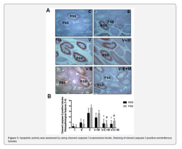
Introduction
Varicocele is an abnormal vascular dilatation of pampiniform plexus, commonly developing at puberty. Although underlying mechanisms remain poorly understood genetic background, anatomical aberrations, incompetence of venous valves, difference between the drainage of left and right testicular veins were suggested in the etiology [1]. As left spermatic vein being longer than the right vein, it is more commonly incurred to increased hydrostatic pressure and dilatation. Compression of the left renal vein between the aorta and the superior mesenteric artery may also contribute to the disturbed intravenous pressure [2].
The prevalence of varicocele varies between 15-20 % in general population and 30-40% in infertile men, and 11-19% of adolescents [3-6]. It was reported that varicocele is a progressive disease and early diagnosis and treatment in youth may enhance fertility potential [7]. Several contributing factors in the pathophysiology of varicocele have been proposed such as higher temperature of testis, the disorder of neuroendocrine system, autoimmunity, accumulation of renal and adrenal metabolites, genetic and epigenetic factors, hypoxia and oxidative stress [8-10].
Varicocele represents a chronic process within the testicle, which is linked to increased reactive oxygen species (ROS) beyond physiologic limits and, subsequently, disrupting sperm membrane fluidity, causing DNA damage and necrosis [11]. Moreover, superoxide dismutase 1, glutathione S-transferase M1 and T1 which are counteracting free superoxide radicals in cells have been reported to be decreased in men with varicocele, that may be important on disturbed sperm parameters [12]. Apoptosis of germ cells was also demonstrated in the pathogenesis of varicocele-related infertility [13]. Clinical findings suggest that surgical repair of varicocele may decrease seminal oxidative stress levels and sperm DNA fragmentation and, thus, may improve sperm quality [14]. Therefore, surgical intervention seems to be a reliable option in the treatment of varicocele-related male infertility, although some controversial reports exist.
Additionally, anti-oxidant medications such as kallikrein, L-carnitine with L-acetyl carnitine, pentoxifylline, coenzyme Q10 have been used to improve the milieu in the testis in men with varicocele [15]. Metformin is a major therapeutic agent in the treatment of type 2 diabetes mellitus as an insulin sensitizer, which decreases hepatic glucose output and increases peripheral glucose uptake. Although its action was not fully elucidated, metformin attenuated intracellular reactive oxygen species and apoptosis in aortic endothelial cells, myocardium, renal tubular cells and testicular cells [16-20].
Aim
Potential effects of metformin on varicocele-induced testicular damage have not been studied in neither humans nor in animal models. Thus, we investigated the impact of metformin on spermatogenesis, testicular integrity, and apoptotic activity in the testis of adolescent rats with experimentally-induced varicocele.
Materials and Methods
Thirty-six male adolescent Wistar rats (6-week-old) were randomly and equally divided into six experimental groups. Surgical procedures were carried out under anesthesia with intraperitoneal injection of ketamine (50 mg/kg). The experimental groups were as follows:
• (C) Control group; no surgical procedure was performed, and testis was examined after removal.
• (S) Sham group, a midline incision was performed, and testis was examined 8 weeks later.
• (V) Varicocele - only group: Experimental varicocele was induced by partial ligation of left renal vein with
Silk suture at the area medial to the insertion of the adrenal and spermatic vein into renal vein as described previously [21].
• (V+M) Varicocele + metformin group: All rats were treated with metformin (300 mg/kg per day by oral gavages) for 8 weeks following induced varicocele.
• (V/E) Varicocele + varicocelectomy group: Varicocelectomy was performed 4 weeks and the examination of the testis 8 weeks after the induction of varicocele. No medication was used.
• (V/E+M) Varicocele + varicocelectomy + metformin group: Varicocelectomy was performed 4 weeks after the induced varicocele. Metformin treatment (300 mg/kg per day by oral gavages) was initiated after the induction of varicocele and continued for 8 weeks. Left testes were examined 8 weeks after the induction of varicocele in all varicocele - induced groups. As maximum apoptotic activity initiates approximately 28 days after the induction of varicocele the procedure of varicocelectomy was performed 4 weeks after the formation of varicocele [22].
Histologic preparation and evaluation
The testicular tissue was fixed in Bouin’s solution (75% picric acid, 5% glacial acetic acid, and 25% formaldehyde) and embedded in paraffin blocks. Sections (5 μm) were formed, deparaffinized, and stained with hematoxylin and eosin. Spermatogenesis was examined in each group using Johnsen’s score (a score of 1-10 was assigned to each tubule regarding epithelial maturation) as described previously [23]. Sections were examined in a random order under a standard light microscope with 10x and 40x magnification by a blinded histologist; unaware of which group each rat belonged to. Histological grading was done by examining approximately 80 randomly selected seminiferous tubules per rat. Thus, a total of approximately 480 seminiferous tubules were scored for each group.
Histomorphometry analysis
A total of 103 randomly selected seminiferous tubules stained with hematoxylin-eosin were analyzed in each group. The presence of round spermatid stage (RSS) and primary spermatocyte stages (PSS) were assessed as described previously and compared among the groups [24].
Immunohistochemical staining for cleaved caspase-3 and ImageJ analysis
Cleaved caspase-3 was used for immunohistochemical staining. Testicular tissue samples were immediately fixed in 10% neutral-buffered formalin, embedded in paraffin, and sectioned (5 μm). Sections were deparaffinized and blocked for endogenous peroxidase activity with methanol containing 3% H2O2 for 10 m. Ultra V Block (Lab vision, Freemont, CA) for 7 m at room temperature. Cleaved Caspase-3 (#9664, Cell Signaling, U.S.) was applied at a dilution of 1: 500 and incubated overnight at +4 °C in a humidified chamber for nonspecific binding. The sections were washed in phosphate-buffered saline (PBS) and incubated with biotinylated horse anti-rabbit IgG (3 mg/mL; Vector, Burlingame, CA) at a 1: 500 dilution for 1 h at room temperature.
Antibodies were detected using a VECTASTAIN avidinbiotin complex (Vector PK 4000) for 30 m at room temperature. Antibody complexes were visualized after incubation with 3,3’-diaminobenzidine tetrahydrochloride (DAB, Bio-Genex, San Ramon, CA.) and were mounted under glass coverslips in Entellan (Merck) and then evaluated under a light microscope. Immunohistochemical staining for cleaved caspase-3 was analyzed by counting 100 seminiferous tubule cross-sections in each group and expressed as the apoptotic index. In each photomicrograph, the following parameter was measured with ImageJ software: expression levels of cleaved-caspase-3 in both groups at round spermatid stage (RSS) of testes. Each of this parameter was measured 3 times for each image and the average of the 9 measurements of each sample was used for the statistical analysis. Histopathological features examined in rats with normal testis and with sham, varicocele, varicocele+ metformin in a subjective scoring (0 - not present; 1 - low grade; 2 - moderate grade; 3 - high grade; 4 - very high grade).
Statistical analysis
Histopathological findings (Johnsen’s score) were assessed by nonparametric Kruskal-Wallis test, and the mean Johnsen’s score was used in the comparison of the groups. Multiple comparisons were made using Tukey’s procedure. p<0.05 was considered statistically significant. Analysis of variance was used for statistical analysis of the apoptotic index among the groups.
Results
Assessment of spermatogenesis
Johnsen’s score was significantly lower in V group (4.14±1.25) compared to C group (9.1±0.3) or S group (9.0 ± 0.2) groups (p<0.05). V+M group had significantly higher score (6.9±0.6) than V group (p<0.05). V/E group and V/E+M group had similar Johnsen scores (8.9 ± 1.02 and 9.2 ± 0.6). These findings suggest that the administration of metformin resulted in 40.6% of improvement in spermatogenesis in rats with varicocele. However, this favorable effect was not observed when metformin was used along with varicocelectomy.
Histological and morphological changes in seminiferous tubules
Histological and morphological changes in the testes of rats were compared via hematoxylin and eosin staining and degenerated tubules (DT) were only detected in V and V+ M groups, not in C, S, V/E and V/E+M groups (Figure 1). Visual assessment of the disorganized seminiferous tubules further supported these findings as seen in Figure 2. Seminiferous tubule degeneration scores were used for quantification of data (Figure 2b). V group had significantly higher scores of RSS and PSS compared to C and S group (2.6±0.8 and 3.7±0.4; 0.2±0.4 and 0.2±0.4; 0.9±0.6 and 0.6±0.7, respectively) (p<0.05). V/E group had significantly lower RSS (0.7±0.8) and PSS (0.8±0.7) scores than V group (p<0.05). V+M group had significantly lower RSS and PSS scores (1.8±0.7 and 2.6±0.7, p<0.05) in comparison to V group, implicating beneficial effects of metformin in rats with varicocele. When compared to V/E group, V/E+M group did not exhibit any difference in RSS (0.6±0.6) and PSS (1.4±0.5) scores, suggesting the absence of additive positive effect of metformin in varicocelectomies rats.
Apoptotic activity
Apoptotic activity was assessed by using cleaved caspase 3 expressions levels, staining of cleved caspase 3 positive seminiferous tubules were shown in Figure 3a. Cleaved caspase 3 expressions were significantly higher in V group (3.5 ± 0.5) compared to C (0) and S (0.2 ± 0.4) groups. V+M group had significantly lower cleaved caspase 3 level (3.0 ± 0.7) than V group. V/E group had lower cleaved caspase-3 expression levels (1.0 ± 0.7) compared to V group. Treatment of varicoceleectomy rats with metformin (V/E+M) did not further reduce apoptotic activity in the seminiferous tubules (1.75 ± 0.43) when compared to the varicocelectomy group (V/E) (Figure 3b).
Discussion and Conclusion
The present study demonstrates that metformin can reduce the extent of testicular damage in rats with varicocele, although having no effect in rats following varicocelectomy Spermatogenesis, seminiferous tubule integrity and the degree of apoptosis were improved using metformin in the presence of varicocele although it was not as remarkable as what was obtained through varicocelectomy. A review of the literature revealed that the impact of metformin on varicocele was not investigated in humans or animal models until now.
Although it is a commonly identified abnormality not all men with varicocele present with infertility. Some intrinsic factors may render some men to become susceptible to varicocele, thus, the best candidates who benefit from varicocelectomy yet to be clarified. Since oxidative stress was shown to be important in the pathophysiology of varicocele some agents have been used to improve the milieu in the testis [1]. A number of anti-oxidant medications have been studied to relieve detrimental effects of varicocele in the testis [25]. These agents have been used either alone or as an adjuvant therapy with surgery. However, surgery remains the treatment of choice and there exists insufficient data to recommend medical therapy in men with varicocele. Barekat et al. [26] reported that administration of an antioxidant agent N-acetyl cysytein as an adjunct therapy improved semen quality following varicocelectomy [26]. Tek et al. [21] demonstrated that vascular endothelial growth factor decreased apoptosis in varicoceleinduced rats as evidenced by diminished caspase-3 positive cells [21]. Both studies showed the benefit of these as adjunct therapy following varicocelectomy. However, in the present study metformin did not enhance the effect of varicocelectomy.
Minutoli et al. [13] demonstrated that neuronal apoptosis inhibin factor and surviving expressions were significantly reduced following varicocele induction and polydeoxyribonucleotide, an agonist of adenosine A2A receptor, administration restored testicular function [13]. Several other studies detected increased germ cell apoptosis in rats with varicocele [21,22,27]. However, in another study, apoptosis was found to be decreased in germ cells in the testes of infertile men with varicocele as compared with normal men [28]. It was speculated that the fixation of testis in formaldehyde might have played a role in the different result. In the present study, cleaved caspase 3 expression was used to assess apoptotic activity and it was found that metformin reduced apoptotic activity in rats with varicocele, whereas no additional effect was observed when metformin was administered after varicocelectomy.
Metformin is commonly used in type 2 diabetes mellitus and polycystic ovarian disease as an insulin sensitizer [29]. Also, it is present in various tissues including myocardium, liver, pancreas, thyroid, adipose tissue, hypothalamus, pituitary, and male and female gonads [19,30,31]. It has been reported that metformin is mainly transported into cells by organic cation transporters as passive diffusion is limited [32]. Although the mechanism of action is not yet fully elucidated recent studies suggested that metformin acts through AMP-activated protein kinase (AMPK) pathway, inhibits the activity of the respiratory electron transport chain in mitochondria, induces epigenetic modifications which in part may explain long term effects and decreases oxidative stress and apoptotic activity [16,19, 33-35].
Male reproductive system utilizes all these metabolic pathways and is prone to be affected by metformin administration [20,36,37]. Metformin was found to stimulate lactate production which is important in the development of germ cells and show an anti-apoptotic effect in rat Sertoli cells [38]. It was also reported that metformin reduced the apoptotic cells and caspase-3 level in rat testis [20]. The findings of the present study are consistent with previous studies that metformin reduced apoptosis in testis with varicocele. Yan et al. [37] reported that metformin improved the semen parameters related to its effects on weight loss, increased testicular weight and reduced testicular cell apoptosis [37]. On the other hand, Tartarin et al. [36] reported metformin at concentration 10 times higher than therapeutic levels decreased testosterone secretion and the number of Sertoli cells in rats when it was administered during pregnancy [36]. Faure et al. [39] reduction in testicular weight and testosterone level were observed in 6-week-old chickens treated with metformin for 3 weeks [39].
Several groups demonstrated that post-operative administration of metformin can exert protective effects in male reproductive function in rat models [40]. Bosman et al. [41] demonstrated that infertile hyperinsulinaemic men could benefit from metformin treatment in combination with an enriched antioxidant diet [41]. Besides, metformin was reported to act as a protective compound when used in the media for cryopreservation of spermatozoa [30]. In conclusion, metformin reduces detrimental effects of varicocele, although no additional benefit is expected following varicocelectomy. Further studies are required to apply metformin for this indication in humans.
#open access journals#peer review journals#Juniper Publishers PubMed Indexed Articles#reproductive medicine#GJORM in juniper publishers
1 note
·
View note
Link
#Juniper publishers#Juniper Publishers indexed journals#Juniper Publishers PubMed indexed journals#Juniper Publishers PubMed indexed articles
2 notes
·
View notes
Text
Functional Selective D2 Ligands for the Treatment of Schizophrenia-Juniper Publishers
JUNIPER PUBLISHERS-OPEN ACCESS JOURNAL OF DRUG DESIGNING & DEVELOPMENT

Abstract
Functionally selective ligands (also known as biased ligands) of dopamine D2 receptors have been considered as not only valuable tools for dissecting the roles of D2-mediated G protein-dependent and independent signaling pathways, but also better antipsychotic drug candidates for neurological and psychiatric disorders including schizophrenia. Consequently, functionally selective D2R ligands have also been increasingly pursued by the biomedical community as promising antipsychotic therapeutics with improved efficacy and reduced side effects compared with unbiased ligands. This review will discuss the recent development in the discovery of functional selective D2R ligands Figure 1.
Introduction
Schizophrenia is a chronic and severe mental disorder characterized by abnormal social behavior and failure to understand reality [1]. Clinically, the disorder manifests with a large variety of symptoms that fall into three categories: positive, negative, and cognitive [2]. Schizophrenia affects about 1.1% of world wide population [3]. Although schizophrenia is not as common as other mental disorders such as anxiety disorder (18.1%) [4], depression (6.9%) [5], and bipolar disorder (2.6%) [6], the symptoms can be very disabling. Therefore, it is often associated with high levels of morbidity and mortality [7]. The average life expectancy of people with schizophrenia is ten to twenty-five years less than for the general population [8]. This is the result of increased physical health problems and a higher suicide rate (about 10%) [9,10].
Although scientists believe that a combination of genetics, environment, and altered brain chemistry and structure may play a role in the development of schizophrenia [11], the exact cause of this disorder is still unknown to the research community. Consequently, there is no cure for this disorder and treatments have been focusing on eliminating the symptoms of the disease. The primary treatment of schizophrenia is antipsychotic medications [12], often in combination with psychological and social supports. While the current FDA-approved antipsychotic drugs are able to reduce the positive symptoms of schizophrenia in about 7 to 14 days [13,14], they have limited efficacy with negative and/or cognitive symptoms [15,16].
Furthermore, antipsychotic medications can greatly lower the patients' life quality by inducing a wide range of motor, metabolic, cardiovascular, and emotional side effects which also lead to treatment noncompliance [14,17]. Therefore, it is of great necessity to develop novel pharmaco therapies which have better efficacies for treating all three clinical schizophrenia symptoms and possess a low profile for side effects.
With all currently FDA-approved antipsychotic drugs target primarily the dopamine D2 receptor (D2R) for their reaction [15-18], it is indicated that opposing dopamine signaling is central for alleviating psychotic symptoms with schizophrenia [19]. Clinical observations have revealed that schizophrenia-like symptoms occur in amphetamine abusers due to excessive dopamine release [20]. Also baseline dopamine levels and stimulated release of dopamine are found to be abnormal in mesolimbic systems of brains from schizophrenic patients [21]. All these evidences have put dopamine receptor, especially dopamine D2R at the center for the development of antipsychotic drug. Antagonists and partial agonists of D2R have been extensively pursued as antipsychotic therapeutics for the treatment of schizophrenia [22,23].
As a member in the big family of G protein-coupled receptors (GPCR), dopamine D2 receptor (D2R) is Gαi/o coupled whose activation inhibits CAMP production [24]. Antipsychotic drugs targeting D2R were originally identified as being able to bind to D2R and regulate CAMP synthesis [18]. Mounting evident from recent studies indicate that D2R signal not only via canonical pathway involving hetero trimeric large G protein, but also via noncanonical G protein-independent pathways with other signaling proteins including, most prominently, β -arrestins [2528]. Most antipsychotic drugs have been found to have both G protein-dependant and G protein-independent actions [28]. The process by which GPCR ligands, including D2R ligands, differentially modulate canonical and noncanonical signal transduction pathways is a phenomenon known as "functional selectivity" or "biased agonism" [29,30].
With functionally selective D2R ligands that can preferentially activate either canonical or noncanonical D2 signaling pathways [31,32], it is thus very clear that the D2R ligands with discrete functional selectivity profiles will be extremely useful for elucidating the key signal transduction pathways essential for both the therapeutic actions and the side effects of antipsychotic drugs [30]. And this understanding will in turn enable the design of better antipsychotic drug candidates, which can ultimately lead to safer and more effective therapies for schizophrenia patients. In this short review article, we will summarize the recent development in the discovery of functional selective D2R ligands for the treatment of schizophrenia.
Functional Selective D2RLigands
Aripiprizole
Aripiprazole (OPC-14597, 1), an FDA-approved atypical antipsychotic drug, was one of the first functionally selective D2R ligands identified [31,33,34]. It has an excellent side-effect profile presumed, in part, to be due to lack of typical D2R antagonist properties. Although aripiprazole was initially described as a partial D2R agonist, on the basis of assays performed in whole animals and isolated tissues [35-37], it was later demonstrated that aripiprazole could behave as a full agonist, a partial agonist, or an antagonist at D2R depending upon the signaling readout and cell type interrogated [28,31,33,38].
The study examined D2R binding properties of aripiprazole as well as the effects of the drug on three downstream D2R- mediated functional effectors including mitogen-activated protein kinase (MAPK) phosphorylation, potentiation of arachidonic acid (AA) release, and D2R internalization revealed that aripiprazole affects D2L-mediated signaling pathways in a differential manner [31]. In the study examining the properties of aripiprazole at D2 like auto receptors by monitoring the changes of dopamine synthesis in adult rat brain striatal minces incubated ex vivo, it was found that alteration of dopaminergic tone by depolarization affected the actions of aripiprazole on D2- like auto receptors [39].
The in vivo study aimed to investigate the effects of aripiprazole on the D2R downstream cAMP-PKA and Akt-GSK3 β signaling pathways suggested that aripiprazole had differential effects on the cAMP-PKA and Akt-GSK3 β signaling pathways in the brain areas [40]. Additional studies examined the activity of aripiprazole in D2R-mediated heterologous sensitization of adenylyl cyclase and cell-based dynamic mass redistribution (DMR). Aripiprazole displayed a unique functional profile for modulation of G proteins, being a partial agonist for Gαi/o and a robust antagonist for G β γ signaling. Additionally, aripiprazole was a weak partial agonist for both heterologous sensitization and dynamic mass redistribution [41].
UNC9975 (2), UNC0006 (3) and UNC9994 (4)
Through a robust diversity-oriented multi-dimensional modification ofthe scaffold represented by aripiprazole (1), Three β -arrestin-biased D2R ligands including UNC9975 (2), UNC0006 (3), and UNC9994 (4) were reported as the unprecedented β -arrestin-biased ligands for a Gi-coupled G protein-coupled receptor (GPCR) [42]. All three D2R ligands were simultaneously antagonists of Gi-regulated CAMP production and partial agonists for D2R/β-arrestin-2 interactions. Importantly, UNC9975 displayed potent antipsychotic-like activity without inducing motoric side effects in inbred C57BL/6 mice in vivo. Genetic deletion of β -arrestin-2 simultaneously attenuated the antipsychotic actions of UNC9975 and transformed it into a typical antipsychotic drug with a high propensity to induce catalepsy.
Similarly, the antipsychotic-like activity displayed by UNC9994, an extremely β -arrestin-biased D2R agonist, in wild- type mice was completely abolished in β -arrestin-2 knockout mice. These results suggest that β -arrestin signaling and recruitment can be simultaneously a significant contributor to antipsychotic efficacy and protective against motoric side effects [42]. Follow-up comprehensive structure-functional selectivity relationship studies (SFSR) focused on four regions of aripiprazole scaffold (e.g. left hand side phenyl region, middle amino region, central linker region, and right hand side bicyclic aromatic region) resulted in more β -arrestin biased D2R agonists [43].
This combined medicinal chemistry and pharmacological profiling approach also provided the biomedical community a successful proof-of-concept for how functionally selective ligands can be discovered. The study designed to test the effectiveness of UNC9975 or UNC9994 on schizophrenia-like behaviors in phencyclidine treated or NR1-knockdown hypoglutamatergic mice showed that the UNC compounds reduced hyper locomotion in the open field, restored PPI, improved novel object recognition memory, partially normalized social behavior, decreased conditioned avoidance responding, and elicit a much lower level of catalepsy than haloperidol [44]. These preclinical results suggest that exploitation of functional selectivity may provide unique opportunities to develop drugs with fewer side effects, greater therapeutic selectivity, and enhanced efficacy for treating schizophrenia and related conditions than medications that are currently available.
Cariprizine (5) and analogs (Compounds 6 And 7)
Cariprizine(5) is an atypical antipsychotic recently approve by FDA for the treatment of schizophrenia and bipolar mania [45]. It acts primarily as a partial agonist for D2R and D3R [46] with higher selectivity for D3R [46,47]. The structure-functional selectivity relationship (SFSR) studies of cariprazine scaffold carried out by Shonberg and colleagues at Monash University was focused on three main portions of the lead compound: the tertiary amine containing "head group", the cyclohexylene "spacer" group, and the tert-butyl carbamate "tail group" [48].
Similar to the SFSR studies of aripiprazole analogs, to assess G protein-related signaling, the compounds were profiled in the D2 CAMP accumulation assay, whereas β -arrestin signaling was evaluated by measuring phosphorylation of extracellular signal-regulated kinase 1/2 (ERK 1/2). In this testing paradigm, cariprazine (5) displayed a 230-fold bias toward the cAMP pathway compared with dopamine. Interestingly, while all cariprazine derivatives disclosed in this letter showed a bias toward the G protein signaling pathway (6), subtle changes of the D2 unbiased partial agonist, a structurally related aryl piperazine reported by Tschammer [49], led to analogues that displayed a strong bias toward β -arrestin signaling such as compound 7. By combining the medicinal chemistry efforts with novel analytical pharmacology methods [50], it was discovered that the nature of the head group, the composition of the tail group, and the orientation, length, and flexibility of the spacer were all important factors for the control of functional selectivity at the D2R [48].
Functional selective D2R ligands with privileged structures (compound 8)
Another comprehensive structure activity relationship (SAR) studies carried out by Szabo and colleagues at Monash University also led to the discovery of novel functional selective D2R ligands [51]. They investigated the determinants of efficacy, affinity, and bias for three privileged structures for the D2R, exploring changes to linker length and incorporation of a heterocyclic unit. After profiling the newly synthesized compounds in two signaling assays (CAMP and pERK1/2), they were able to identify and quantify determinants of functional selectivity at the D2R. The results from combined medicinal chemistry and pharmacological profiling approach revealed that: 1) substitution on the phenylpiperazine privileged structures (2-methoxy vs 2,3-dichloro) influenced bias when the thienopyridine heterocycle was absent; and 2) upon inclusion of the thienopyridine unit, the substitution pattern (4,6-dimethyl vs 5-chloro-6-methoxy-4-methyl) had a significant effect on bias that overruled the effect of the phenylpiperazine substitution pattern [51]. This latter observation could be reconciled with an extended binding mode for these compounds, whereby the interaction of the heterocycle with a secondary binding pocket may bring functional selectivity to the parent compounds. The resulted novel D2R partial agonists, 8 and 9, display a similar affinity for the D2R as aripiprazole but exhibit distinct functional selectivity profiles, which made them useful tools to explore the contribution of functional selectivity to antipsychotic efficacy.
Functional selective D2R/D3R partial agonists
Dopamine D2R and D3R are known as valuable targets for the treatment of neurological and psychiatric disorders including schizophrenia [52-54]. Hiller and colleagues evaluated a series of newly synthesized compounds for their ability to differentially activate distinct signaling pathways [55].
Measurement of D2L- and D2S-mediated [35S] GTPyS incorporation in the presence of coexpressed Gao and Gai subunits showed significantly biased receptor activation for several test compounds [55]. A follow-up study from the same group using the same evaluation methods yielded the most striking functionally selective D2R ligand, carbaldoxime 8b (9, Gaol, pEC50 = 8.87, Emax = 65%; Gai2, pEC50 = 6.63, Emax=27%) [56]. It was also indicated in the study that 1,4-disubstituted aromatic piperazines (1,4-DAPs) behaved as antagonists for β -arrestin-2 recruitment, implying significant ligand bias for G-protein activation over β -arrestin-2 recruitment at D2R. Regiochemistry and the nature of functional groups attached to the pyrazolo [1,5-a]pyridine moiety strongly influence ligand efficacy and selectivity between D2R and D3R activation [56].
Other functional selective D2 ligands
Intensive structural exploration on aripiprazole scaffold engendered UNC2438 (10) which was found to be a G-protein biased compounds [57]. Further structure-functional selectivity relationship studies (SFSR) on UNC2438 focused on the right hand side benzothiazole moiety and the left hand side phenylpiperazine moiety furnished a few additional G-protein biased compounds which were partial agonists in D2R Gio- mediated CAMP inhibition assay and simultaneously inactive in D2R-mediated β -arrestin-2 recruitment assay [57].
Most recently, a tailored virtual library with close to 13,000 compounds bearing 2,3-dichlorophenylpiperazine, a privileged orthosteric scaffold, connected to diverse chemical moieties via a linker was docked to the D2R model [58]. Eighteen top-ranked compounds that occupied both the orthosteric and allosteric site were synthesized, leading to the discovery of 16 partial agonists. While a majority of the ligands had comparable maximum effects in the G protein and β -arrestin recruitment assays, some displayed preference for a single pathway. In particular, compound 11 stimulated β -arrestin recruitment (EC50 = 320 nM, Emax = 16%) but had no detectable G protein signaling.
Conclusion
The growing realization of the complexity of G protein coupled receptor (GPCR) mediated signal transduction pathways, specifically D2R mediated signaling pathways, has provided a theoretical framework for the development of functionally selective or biased ligands. Several studies have demonstrated that agonists differ in their ability to activate various pathways. Notably, blockade of β arrest in recruitment was found to be a shared property of antipsychotics that exhibit either antagonist (e.g., haloperidol), or partial agonist (e.g., aripiprazole) activity through Gai/o-CAMP pathways [28]. In contrast, a study with analogs of the novel antipsychotic aripiprazole suggested that D2 ligands with Gai/o antagonist and β -arrestin agonist activity may have antipsychotic behavioral activity with reduced extra pyramidal side effects in a mouse model [3]. While there are still a lot of questions to be answered in this field, heightened awareness of the potential benefit of pathway biased D2R ligands has inspired scientists in this area develop more functionally selective D2R ligands as better antipsychotic therapies for schizophrenia.
For more Open Access Journals in Juniper Publishers please click on: https://www.crunchbase.com/organization/juniper-publishers
For more articles in Open Access Novel Approaches in Drug Designing & Development please click on: https://juniperpublishers.com/napdd/index.php
For more Open Access Journals please click on: https://juniperpublishers.com
To know more about Juniper Publishers please click on: https://juniperpublishers.business.site/
1 note
·
View note
Text
Juniper Publishers-Open Access Journal of Case Studies

A Case Study on Birth Experience
Authored by Ayman Aboda
Abstract
Background: Normal consciousness may be profoundly changed during labour. Access to heightened states of personal and existential awareness may be part of the uninhibited ritual of natural childbirth.
Aim: Validate the possibility of heightened awareness and transcendence that can occur beyond the province of normal human experience. Peek experiences may bring life changing realizations of deep universal connection and personal insight.
Findings: Breakthrough experiences may occur in any state of intense physical focus, including the mindfulness of supported birth practices.
Discussion: The perspective reiterates the importance of rational, individualized, woman-centred care in birth.
Conclusion: The environment of birth, the safety and support of known and trusted care givers can allow birth events to unfold with the least possible intrusion. A hitherto under-recognized sequalae for such freedom may be the possibility of connecting to a state of expanded awareness that can bring profound unveiling of inner being and self-acceptance.
Keywords: Normal consciousness; Natural childbirth; Woman's emotional experience; Bleeding; Fearfulness; Birth experience; Acute medical resuscitation, Neurosurgeon
Statement of Significance
Problem
Constrictive models of care during birth.
What is already known
Current institutionalized models are driven by risk and litigation. Success in mitigating such harms has been tempered by spiralling costs of intervention and more insidiously, a diminution of the birth experience.
What this paper adds
The rationalization of appropriate care. The importance of choice and the understanding that birth can yield of itself, a glimpse into the extraordinary, an experience of wonder and life changing self-awareness that can be truly transformative for the mother and for all those with whom she shares her journey.
Go to
Pushed to the Limit - Reclaiming the Ecstasy of Birth
“I remember when my world changed forever. I experienced something miraculous when I gave birth, I gave birth to myself as a mother. During labour, I noticed the world around me change. The lights seemed dimmer and there was a silence in the room. I was conscious but it felt different. There was an incredible sense of calm. I could sense everything, the bed, the room, my breath, and heartbeat, my thoughts and feelings. Time stood still. I was no longer connected to the room. I was distant in a place I had never been before. I was totally removed from everything. There was a sense of floating without boundaries. It was so calm, peaceful. I remember looking down as I hovered over my body, watching myself from above, as if I were two separate beings. I felt so loved. Fearless. I have never felt like this before, the beauty, the purity and bliss. A realisation of my existence came. It was as if I had gained clarity and the answer to life's many questions. Everything was exposed in its truest form. I knew why I was here and what I was born to do. I was here to create.”
GS – personal birth story.
What’s it like?
Long before the infamy of Covid 19, a philosopher once asked what it would be like to be a Bat? [1] Would it think as we do? Would it experience the world in the same way? Of course, we imagine that it would, but then all we’re really doing is putting ourselves within, thinking of it as just a smaller version of us; something that sees as we do, hears in the same way – albeit with bigger ears, and otherwise makes sense of its perceptions with the same quality and perspective of mind. But no one can really say for sure – which was in fact the whole point of the question: to remind us that all we can ever truly know is what it’s like to be us. And what is that you might then ask. Well, that’s easy, it’s the awareness we have of living, of being here, experiencing the world around us and knowing where we are within it. Now whilst this may or may not be true for other creatures - including bats, the outward-looking, body-centred perspective through which we frame our experience of living seems so much a given norm, that it’s hard to imagine there could be any other way of doing things. But is there?
Looking beyond the veil
In his book, “Life after Life”, Raymond Moody described a near-death experience which was noted following an acute medical resuscitation [2]. The survivor told his rescuers that whilst they’d been busy trying to save him, he’d been looking down as things occurred, watching the entire scene unfold from a point that was from somewhere outside his body. On the one hand he knew that this was something that shouldn’t normally happen and yet it had seemed so undeniably real that he couldn’t believe it hadn’t. More recently, American neurosurgeon Eban Alexander reported a similar sensorial shift with translocation of living awareness away from the body at a time when deep, septic coma had stopped all measurable brain activity [3].
These and other accounts suggest that the seat of consciousness may not be as firmly anchored as previously imagined, and that the usual, body-centred perspective may be just one of many possibilities available to us. But of course, we know this already for in our dreams each night, most of us experience vast multiplicities of non-ordinary awareness or altered states of being that we simply take for granted as flights of fantasy. In his book, “Journeys out of the Body,” Robert Monroe described specific techniques to intentionally induce similar states of transpersonal, or Out-of-Body Experience (OBE) in daytime too, where consciousness could exist replete and fully visceral despite separation from the physical body [4]. Cognitive awareness of self and surroundings remain corporally vital, with the experience most often described as a heightened or more splendid state of normal which could at times lead to an unprecedented feeling of bliss or profound belonging as if having become intimately connected to some greater universal presence or unconditional ease.
Not surprisingly, Out of Body Experiences can transform lives, and indeed they do. For the prophet Elija, the apostle Paul, Saint Francis of Assisi, the Buddha, and the modern spiritual teacher Ekhart Tolle, this was powerfully so. Sadly however, such revelations seem sparsely scattered, contained if lucky, to the zeal of a few determined practitioners or else the fervour fuelled of religious rapture or tribal ceremony such as the dreamtime of indigenous Ngangkari or shamanic ritual or more illicitly, from the psychedelic haze of contemporary drug culture. Without the agency of such provocateurs, one might reasonably wonder if the phenomenon was indeed meant to happen in normal life. Afterall, nature tends only to preserve or promulgate those behaviours that best suit the ability to survive - including the way we perceive the world. The paucity of OBE’s, notwithstanding their reputed glimpse of wonder, may simply reflect that they are less advantageous at keeping us alive - unless of course something changes that makes them more able to do so.
Holocaust survivor Viktor Frankl described looking down at his body during the terror of war and internment [5]. He thus felt distanced from the inhumanity and outrage of the horrors inflicted upon him and was somehow more able to survive. To withdraw from the immediacy and acuity of the senses can help to endure, to sustain trials of physical hardship and duress. Similarly, to quell the plethora of the senses, to focus intently may optimize performance in peek states and zones of intense concentration allowing an almost trance like state of deep attention for what needs to be done. In such states, the extraordinary can become possible and feelings of deep, transpersonal connection and grounding can arise.
Pushing to the limits –the energy of childbirth
“In the most intense hours of labour, I became mindless, floating in boundless space between contractions. All thoughts receded. My mind plummeted into an immense silence bathed in love and well-being. I felt a oneness with all mothers who had ever birthed” [6].
A woman's emotional experience during labour may show common themes, beginning with excitement and a need to feel safe and supported as her contractions develop which means she can then focus her energy on getting through things, one surge at a time [7]. Her world then narrows as concentration deepens and she may become less aware of things around her, moving into a ‘zone’ of timelessness, of dissociation or disconnection with the rest of the world. In this phase, perhaps 10% of women may experience states of altered awareness, including fully-fledged OBE’s where the boundaries of self and ordinary reality become less defined and deeper, more subtle levels of creativity and spiritual encounter can occur. These feelings then transition and become more grounded as an urge to push strengthens and a reconnection with the present emerges, often bringing a realization of awe and amazement as the power of their bodies moves them irresistibly towards birth [8].
modelling
“In achieving the safety of childbirth our society may have lost more than it has gained.” [9]
Birth however is not always perfect. Whilst it is a natural process, left to itself, it may not always lead towards a desired or safe ending. There may be pain, unprecedented in its intensity; bleeding, a fearfulness of what lies ahead, of what remains unknown or unexpected. There may be escalating risk or concern that must be managed. Models of care have thus evolved to mitigate, to wrestle control from such uncertainty, to bring order to chaos, to reign-in the freedoms of nature’s way. And so, we change. We change things, and more sadly so, we change ourselves. We stop seeing women as mothers or as mothers-to-be; they become patients. We take them from home, from community and on-country, and admit them to hospital to be cared for, to be monitored, to be made right. Labour becomes a diagnosis, an illness, a condition that must be treated and fixed. Natural rhythms are ignored and give way to ever more intrusive cascades of intervention.
Without doubt, neonatal and maternal outcomes have improved, but there comes too a growing apprehension of cost, of over-service, and more distressingly, an ever-widening wound of visceral and emotional discontent that follows thereafter. What began in good faith, what began because we genuinely care, because we wanted to help, has become a mandate. We now do what we do because we feel we have to. We feel we must. We believe it’s best. But is it always so?
By institutionalizing the birth experience, we can diminish a woman’s ability to participate, to help nurture the power and flow of her body to progress naturally and spontaneously. More subtly, by controlling her experience so arduously, we hide from her the opportunity to encounter an intimate, perhaps sacred awakening of deeper self that might otherwise have occurred. We thus sterilise the possibility of transience, of enchantment. We diminish the extraordinary to something best forgotten. We brush it aside as vagrant, a symptom of momentary dysfunction, or the rekindling of aberrant memory in the fever of fatigue [10].
Pushing back - reclaiming safe passage
Birth is of itself complete, it lacks nothing to make it more so. We have tried to make it better and of course in many ways we have, but at what cost? And for such gains won, how much has been lost? In our desire to make it fit, to conform to modern standards, there may be much that we have taken, that we have forsaken. We may have stolen from it something subtle, an opportunity to transcend normal living and experience an intimate revelation of profound connection and wonder.
The awareness we have of ourselves in the physical world is miraculous, a perspective made possible by the wondrous workings of what makes us human. Occasionally however, states of expanded, other-worldly consciousness can occur, where glimpses of a far-from-normal reality can pervade our senses with life changing ardour. When we consider the impact that such transformative experiences can bring, we may well grieve for their paucity.
In Australia, over 300 000 women give birth annually. 1 in 10 of these may experience feelings of altered consciousness which for some, may lead to an encounter of unprecedented personal realization and bliss. Imagine the impact that such life-changing experiences could bring. Imagine a birthing space where the unfolding of such deep ritual was nurtured, where we protect and gently support each mother to follow if she desires, the natural rhythms of her body. Where we gave freedom to experience the power of birth, and, if it should happen, the revelation of divine inner being that may enrich her life thereafter. Imagine what this would bring for her little one as she bonds and for those with whom her life is shared. Imagine what this would do to her world. To yours. To ours. It’s not just a want, it’s a rite worth wanting, a rite worth reclaiming. All we need do, is just let it happen. I think we can.
To know more about Juniper Publishers please click on: https://juniperpublishers.com/manuscript-guidelines.php
For more articles in Open Access Journal of Case Studies please click on: https://juniperpublishers.com/jojcs/index.php
#Juniper Journals#Juniper Publishers Indexing List#Obstetrics and Gynaecology#Pediatrics#Transplantation Medicine#Rheumatology#Molecular Biology
0 notes
Text
Influence of Moisture, Temperature and Microbial Activity in Biomass Sustainable Storage. Special Focus on Olive Biomasses
Abstract
Biomass is a renewable energy source that, due to its high seasonality, needs to be stored, handled and managed in suitable conditions for its optimum use. Sustainable storage is, therefore, a key process in which biomass can lose much of its qualities as fuel. The article presents an exhaustive bibliographic review of the factors that affect the quality of biomass during storage and the interactions that occur among them. Humidity, type of product, granulometry, size of the stockpile, airflow, temperature, and microbial action are analysed as the main factors affecting biomass during storage, and the results are compared with the tests that have been carried out on biomass from olive groves and olive oil industry. Recommendations are presented so that, using a correct storage method, losses, degradation and self-ignition risks are reduced and the energy quality of the fuel could be improved, taking advantage of the storage process to optimize the net energy yield.
Read More about this Article: https://juniperpublishers.com/ijesnr/IJESNR.MS.ID.556165.php
Read More Juniper Publishers Google Scholar : https://scholar.google.com/citations?view_op=view_citation&hl=en&user=4WXzQFMAAAAJ&citation_for_view=4WXzQFMAAAAJ:EUQCXRtRnyEC
#Juniper Publishers PubMed Indexed Journals#Juniper Publishers Google Scholar#waste management#environmental engineering#natural resource management
0 notes
Text
Impact of Cover-Crop Residuals on Soil Carbon Sequestration and Respiration- Juniper publishers

TGlobal policies encourage to lower greenhouse gas emissions in order to maintain climate change under the limit of +2°C at the horizon 2100. An important part of these gases are emitted from croplands and farms [1]. To reduce the environmental impact of croplands, diverse techniques and practices have been widely used by farmers, based on conservation agriculture (simplified cultivation techniques, cover-cropping, agroforestry, etc.). The use of these techniques has been adopted freely, according to the good will of farmers. Scientists have broadly studied these crop management practices in order to evaluate their impact on climate change [2–4]. Actual assessment of carbon emissions and storage capacities of croplands under such crop management practices had helped us to discriminate the practices useful for carbon accumulation. No-tillage has an important role to play in agriculture, mainly because of the great impact on soil bulk density and ease of crop germination. However, it is now well known and admitted that no-till have no significant impact alone on soil carbon storage capacities over the entire soil profile [5]. Cover-cropping is also an interesting and promising management practice to consider when accounting for climate resilient agroecosystems, soil carbon sequestration [6] and ecosystem services [7]. This practice can have very contrasted impacts on soil and the agroecosystem depending on sowing and destruction period, species used, for how long and how the residues are managed. Indeed, cover-cropping leads to improved biomass production and undoubtedly, to more crop residues. The impact of crop residues on soil carbon have been widely studied [8–10], but their impact on soil respiration still needs to be clarified. How do cover crop residues respiration change over the crop season? Soil respiration was measured with an infrared portable gas analyzer together with a soil respiration chamber (EGM4 and SRC1, PP Systems, Amesbury, USA). The study site was located in Southwest France (N 43° 24’ 38.057’’, E 0° 17’ 17.612’’, alt= 266 m) on a soil defined as a Stagnic Luvisol according to the World Reference Base for Soil Resource [11]. No-till and cover-cropping have been implemented for 20 years, which improved soil organic carbon content of 48.8% compared to conventional agricultural system. The cover crop was mainly composed of faba bean (Vicia faba), oat (Avena sativa) and triticale (×Triticosecale) for the last 4 years. We measured soil respiration with and without residues and for residues alone. We observed an increase of soil residues respiration over the season as well as of values dispersion (Figure 1). Very low level of respiration rate was observed from the 30th of June to the 10th of September, even if few points had respiration values in the range of values generally observed for soil respiration for temperate ecosystems [12]. But significant higher values of respiration were observed on the 29th of September and October (p value < 0.05). The increase in soil respiration across the season was attributed to the maturation of crop residues and their gradual transformation from fresh organic matter to labile and dissolved organic matter, more easily degradable for microorganisms. It then appeared that the degradation process of cover crops passed through different phases; slow degradation until the senescence of the cash crop (here maize), then degradation inducing significant respiration. It seems that maize senescence leaded to favorable conditions for cover crop residuals degradation. Usually, when maize enters senescence, farmers stop irrigation to let maize dry before harvesting. Cover crop residuals could reach their optimum degradation rate with optimum both soil moisture and temperature promoting respiration of residuals in this particular time period. A second hypothesis is that maize plants senescence could imply microorganisms within maize rhizosphere to look for other sustainable carbon source when maize roots stop to diffuse exudates in soil [13,14]. These microorganisms could change of substrate when maize exudates stop and move from exudates to surface carbon.
Conclusion
TCover-crops constitutes a good solution to improve soil carbon content sequestration, both by increasing biological activities notably through biomass accumulation and exudation, and abiotic impact on cropland (temperature and humidity control). However, the production of supplementary biomass induces supplementary carbon fluxes from the agroecosystems that needs to be taken into account when assessing carbon footprint of croplands.
To know more about Journal of Agriculture Research- https://juniperpublishers.com/artoaj/index.php
To know more about open access journal publishers click on Juniper publishers
0 notes
Text
Power Estimates of Coastal Zone Winds and Waves via Box, Whisker and Outlier Distributions at Atlantic Eastern Seaboard and Pacific Ocean Energy Sites- Juniper Publishers
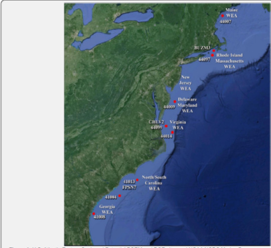
Abstract
The U.S. Bureau of Ocean Energy Management (BOEM) has a congressional mandate and the U.S. Department of Energy (DOE) both have mandates to assess oceanic wind and oceanic wave energy and power resources and impacts; both structural and potentially ecological. Oceanic offshore winds and waves are viewed as being relatively steady sources of energy. However assessments of the amount of the wind resources and wave resources in U.S. coastal and oceanic environments have not been evaluated and have only been estimated by several rudimentary modeling efforts. As such, there are many National Oceanic & Atmospheric Administration (NOAA) National Data Buoy Center (NDBC) Marine Buoys which have collected considerable data on both wind and waves that can be harvested and evaluated for in-situ observations. Also the U.S. Department of the Interior, Bureau of Safety and Environmental Enforcement (BSEE) is charged with the development of hazard curves for wind energy areas off the Atlantic Seaboard. As such BOEM has several proposed U. S. Eastern Seaboard, Atlantic Ocean energy/power sites. Likewise DOE is interested not only in potential Atlantic sites, but Pacific sites as well. In this manuscript we captured several representative time series of winds and waves from NOAA buoys, and evaluated those sites for their oceanic wind energy and wave energy potential, by employing a basic statistical methodology. The data sets are very self-consistent, and levels of energy vary as a function of locale, monthly, seasonally and annually. While ecological studies are called for at BOEM sites, such as on fisheries and other living marine resources, those are beyond the scope of this study.
Introduction
The U.S. federal agencies BOEM and DOE are committed, by law, to assessing oceanic wind and wave power. Wind power ensues from the flow of air through wind turbines to mechanically power generators for electricity. Wave power results from oceanic surface gravity wave (SGWs) passage through ocean based turbines to mechanically power generators for electricity. Wind and or wave power, as alternatives to burning fossil fuels, are plentiful, renewable, widely distributed, clean, and produce no greenhouse gas emissions during operation. The net effects on the environment are far less problematic than those of nonrenewable power sources. Wind farms consist of many individual wind turbines which are connected to the electric power transmission network. Offshore winds and waves are generally viewed as being steadier sources of energy than are land based sources, and far offshore farms are conceptually envisioned as having less visual impact than land based farms, but construction and maintenance costs are considerably higher than on land. Wind and wave power are believed to be very consistent from year to year but also to be characterized by significant variation over shorter time scales as SGWs are driven by winds which have great variability over “meso” hourly to daily to weekly temporal scales and spatial scales of kilometers to 10’s to 1000s of kilometers. The SCPC is one such public utility that has an expressed interest in coastal energy.
In Figure 1, we present the Wind/Wave Energy Sites (WEAs) that are of interest to BOEM and DOE. Figure 1 also shows the locations of the NDBC Marine Buoys. NOAA maintains a national coastal and oceanic based network of marine buoys described at the National Data Buoy Center (NDBC) at: http://www.ndbc.noaa., and the data are available from the NOAA National Centers for Environmental Information (NCEI) at: http://www.ncei.noaa.gov/. The data are available in a digital format and are quality assessed.
In Figure 2, examples of oceanic wind and wave energy harvesting systems are presented. As shown in Figure 2a (left panel), offshore wind turbines are subject to oceanic forcing and as such could be damaged or destroyed by exceptionally robust oceanic winds and or waves. Figure 2b (right panel) depicts an underwater configuration of a wave power system. We note that the depictions of wind and wave power generating devices shown in Figures 2a, 2b, are just two of the many that the engineering community has designed, produced and tested (for example: Falness [1], Twidell et al. [2], McCormick [3] Cruz [4]). Variability of winds and waves are well known to mariners and as such it is of value to assess the observed variability of winds and waves in the vicinities of the proposed BOEM lease sites.
Data
The NDBC Marine Buoy wind speed data are sampled every minute while he surface gravity wave data are sampled every second. On a twelve hourly basis the data are uploaded to the NOAA GOES satellite constellation and then downloaded to the National Aeronautics and Space Administration (NASA) Wallops Island Virginia receiving stations, then transferred to and checked for quality at the NOAA NCEI in Asheville NC, and subsequently archived into the NCEI archives. Other atmospheric and oceanic state variable data are also collected but are not dealt with in this report.
Statistical analyses of weather and climate state variables have often focused on averages of the atmospheric and oceanic variables, such as record length mean wind speeds or mean wave amplitudes or some kind of continuous or box-car or rolling averaging of the various time series [5]. However, the means and departures from the mean are also of interest in the realm of renewable energy. In addition to a determination of the wind and wave potentials for producing sources of renewable energy [6], as mentioned above, there are also agency and industry concerns about deploying expensive structures in and on the ocean in areas where there could be naturally occurring excessively high winds and or very large amplitude waves that could destroy those structures [7]. As such, the totality of the various time series contain the complete signals of wind speeds and wave amplitudes, but in actual fact, the time series look very noisy in raw time series format and various methods have been used by investigators to separate the “signals” from the “noise” [8].
In attempting to separate signal from noise, this study consists of a statistical decomposition of the distribution of atmospheric winds and oceanic surface gravity waves collected by NOAA NDBC Marine Buoys, in the vicinity of the BOEM sites in the Middle and South Atlantic Bights (MAB and SAB, respectively). The NDBC sites were selected by their locations near BOEM and DOE potential sites. The study considers wind speeds and wave amplitudes in a descriptive statistical manner using what are called box plots. A box and whisker plot is a convenient way of graphically depicting groups of numerical data through their central 50% distributions, their medians (their “boxes”) and nominally their upper and lower quartiles (their “whiskers”). Our box plots also have crosses extending vertically from the upper quartile whiskers, which we take to be about 23.5% of the uppermost observations, indicating 1.5% variability above the upper 98.5% of the observations of a particular time series record. Thus we invoke the term of box-andwhisker- and–outlier (B&W&O) plot.
Outliers in the upper several percent of the upper quartiles are plotted as individual points and signify individual observations of relative extreme magnitudes. Box plots are non-parametric in that they display variation in samples of a statistical population without making any assumptions of the underlying statistical distribution. We present our decomposition plots as a function of month by year and wind speeds and wave amplitudes as a function of year by month. The variability of winds and waves from site to site, over the years at a specific site, and by month at a specific site can be considerable. We also have duplicate plots of the outliers, in which we have connected the outliers to provide a better visual sense of the extreme observations. The data can be used to validate numerical model output by individual atmospheric event, by clusters and or families of atmospheric and or oceanic events.
Methodology
The methodology used to decompose the NDBC Marine Buoy data sets is commonly referred to as Box and Whiskers or “B&W” (Bendat and Piersol, 2000) decomposition. The B&Ws basically and to lowest order decompose the data into the percent (%) of the total distributions recorded at the sites in terms of their 50% overall central amplitudes, about which there are upper (25%) and lower quartiles (25%) centered about the medians. The medians are contained within the 50% “boxes”. Then there are the upper and lower amplitude quartile “whiskers”. Within an as an extension of the whiskers, there are extreme event signatures or “outliers”; both below and above the lower and upper whisker quartiles. Again, these represent extremely low and extremely high amplitude events.
Here is what is done mathematically to compute the Boxes and Whiskers (and “Outliers”); (B&W&Os):
(1) Calculate the height of the box (Y coordinate of top - Y coordinate of bottom). This is called the «interquartile range» as it is the distance between the 75th and 25th percentile (first and third quartiles);
(2) Above and below the box, draw whiskers of length 1.5 times that interquartile range; and
(3) Plot any points beyond the whiskers as potential outliers or extremely high amplitude events, relative to the particular distribution of observations at a specific site.
In the plots to follow, there are many potential outliers above, but not below the whiskers. That would suggest, for example, if one were modeling wave height versus wind speed or some other variable, we would put wave height on a logarithmic scale to make it look more symmetric and normal. It could well be that if we did the B&W on a log (wave height) scale; we would have many fewer “outliers”. As these “O’s” represent valid data, there is no need to make the data distribution appear to look normal. As was pointed out by Gladwell [9], an “outlier” is a statistical observation that is markedly different from the others of the sample. Thus, the B&W&O methodology does an excellent job in distinguishing those singular data points
If we have a distribution, one that is normal for example, we can calculate the theoretical endpoints of the whiskers. There will remain some probability of being beyond those endpoints; maybe it might be only 0.001. Now if we were to have, say, 1 million points you would expect to have (0.001) X (1,000,000) = 1000 points beyond those whiskers, that is, there is no adjustment for sample size. Even in a perfect theoretical distribution, given enough points, some will fall outside those whiskers. So we now look at the distributions of the wind and wave amplitudes and describe the distributions derived from the NDBC Marine Buoys.
We will first present an example of a B&Ws plot for one day from NDBC buoy 41004 offshore of Charleston South Carolina (SC). That day Figure 3 is 13 September 2005 during the passage of Hurricane Ophelia. 50% of the winds recorded on that day were between 4 and 9.5 meters/second (m/s) with a median of 7m/s. The lower quartile is between 0 and 4m/s. The upper quartile is 9.5 and 17.5m/s. As it occurs, in 2005, 20 of the top 22 observations between 18 and 23.5m/s that would be considered outliers occurred during the passage of Ophelia. The other two were likely wind gusts which occurred prior to the formal arrival of the hurricane, and on the same date.
In Figure 4 we see the wind amplitudes at the same site from 1978-2005. Clearly, hurricanes have contributed a significant share of the most extreme outliers recorded at site 41004, off of Charleston SC, over the 18 year period. However there are many other dates when significantly high winds were recorded; even in excess of 30m/s. SC is at the southernmost extent of the zone of the genesis of Extra - Tropical Cyclones (ETCs), a zone centered about Cape Hatteras North Carolina (NC). We will look at this more in depth as we consider wind amplitudes by moth later in the text. The Years 1978, 1981 and 1986 had relatively few extreme events. We note that there are many years without complete time series; a hazard of marine buoys that, being subjected to harsh oceanic conditions, often break down and are left non-serviced for lengthy periods of time; as NOAA must schedule vessels to assess damage and provide service of either repair or replacement.
In Figure 5, we see the wind speed distributions (in percentage (%) of total) shown in Figure 4 as a function of frequency (in wind speed/day). As we can see, the complete suite of observations of wind amplitudes over a total period of 18 years, assume the distribution of a log normal function. The lower quartile, 50% middle, the upper quartile and the outliers, shown as blue crosses and flags, are also shown.
In Figure 6 we present the surface gravity wave amplitude observations from NDBC buoy 41004. Wave heights are presented in units of meters and the numbers on the blue crossed outliers indicate the specific months during which those relatively high amplitude waves were measured. Years 1999, 1996 and 2001 were especially high energy years with most extreme events in 1996 having occurred in September, thus related to hurricane passages while during the month of March in 2001 due to Mid-Latitude cyclone passages.
Figure 7 displays the wave amplitude distributions (in % of total) shown in Figure 6 as a function of frequency (in wave heights in units of meters/day). As we can see, the complete suite of observations of wave amplitudes over a total period of 16 years, assume the distribution of an exponential function. The lower quartile, 50% middle, the upper quartile and the outliers, shown as blue crosses and flags, are also shown.
The annual distributions of wind speeds and the wave amplitude distributions are in solid agreement. However it is clear that wave amplitudes are not only a reflection of the local generation of waves (“sea”) but also carry the arrival of waves which have been generated elsewhere (“swell”) and which have propagated into the area of the buoy and thus contribute to the overall wave amplitude measurements. Curiously the spectral distributions of the wind speeds Figure 5 and that of the wave amplitudes Figure 7 appear to be “log normal” in the winds versus “exponential” in the waves. The reasons for this are not presently known and this could be a universal finding. The peer reviewed literature contains no reference to these results and thus original findings. It is herein speculated that momentum inputs from atmospheric winds are non-linearly transferred into wave momenta.
We now look at the archived records of wind speed and wave amplitude data collected on NDBC buoys in the areas of interest to BOEM and DOE and shown in Figure 1. For example, in Figure 8 we consider the time series, data length plots of monthly wind speeds and wave amplitudes at Station 44009, by way of example close to a potential BOEM and DOE site off Chesapeake Bay, Virginia.
In Figure 8 we see that there were many periods of missing data, as is not uncommon with Marine Buoy data; particularly wave data. For NCDC 44009, the missing wind data months are Jan 1985, Jan-Feb 1986, Dec 1988, Feb 1989, Jul 1990, Jan - Apr 1991, Dec 1992 - Apr 1993, Oct 1995, Nov 2004, Dec 2008 - May 2009, Mar - May 2010, Sep - Dec 2013. All other months are complete. At NCDC 44009 the missing data months for waves are Dec 1988, Nov 1992 - Apr 1993, Jan - May 1994, Oct 1995, and Jan 2013. All other months are complete. The missing months were linearly interpolated with straight lines; which leave one with the impression of coherency. This latter exercise was straightforward but not without mathematical challenges; if it were to be done properly. However that is beyond the scope of this report, which is informational in nature and content. In general and for the most part, the wind speed and wave amplitude data track closely, with the appreciation that while the wind field is “local”, the wave amplitude field consists of near-field locally generated waves or “sea” and farfield or “swell” which propagates into the measurement domain. As shown (in a representative example), the monthly mean winds range from 4 - 10m/sec and monthly mean wave amplitudes range between 0.5 - 2m, both with highs in January – March and lows from June - August. Overall, the monthly averaged wind speeds and wave amplitudes at all of the NDBC stations shown in Figure 7, are highly visually positively correlated in keeping with the Figure 8 so are not shown here.
We next consider the B&Ws by month for all years averaged together for wind speeds, location, versus their wave amplitude counterparts for NDBC Marine Buoy 44009, are presented by way of example in Figure 9.
In Figure 9, the medians and 50% “boxes” of both wind speeds and wave amplitudes reach annual minima from June – August and both peak over the period of November – March. This is not so evident in the more conventional time series plot shown in Figure 8. In Figure 9, upper quartile (dotted line “whiskers”) and outliers (red crosses) are highest in August and September, reaching 30m/s, associated with the infrequent but highly energetic passages of hurricanes (we note that in the Figure 5 representation of years by month, the month of September is most prominent), followed by November and January – March, reaching 25m/s, associated with the frequent passages of ETCs. Wave amplitudes are in-kind, reaching 7.5 – 9m in winter and only 7m in September, unlike the 41004 counterpart which reached 13.5m in September (Figure 5). This description is not in the least evident in Figure 8. Thus we conclude that there is substantial informational content of a different kind in the representations of B&W&O winds and waves presented in Figure 9.
In a complete sweep we decomposed the time series of wind speeds and wave amplitude observations at the NOAA NCDC Marine Buoy Sites near the BOEM and DOE sites, as shown in Figure 1, into B&W&Os by individual month as a function of years and by individual year as a function of months. The year to year variability, month to month and site to site variability in distributions was considerable and will be summarized next. Unfortunately several of the sites lacked wave data and several of the sites had time series that were abbreviated in length. To provide the most comprehensive overview, we present the winds and waves at the northernmost site, 44007, a central site, 44009, and the southernmost site 41008; as these three stations had the more complete time series. These are presented in Figure 10, by months averaged over the years of the composite time series records. The outlier data, which appear as the red crosses above the “whiskers” in Figure 10, are captured within upper and lower solid lines for better visualization moving from month to month and between buoy sites as a function of buoy location. The topmost left and right upper panels are data from Maine (ME), the middle left and right panels are from Delaware/ Maryland (DE/MD) and the lower panels are from Georgia (GA).
In Figure 10, we see that in general, 50% of the wave amplitude data are between 0.5 and 1.5m at all sites for all months, with annual lows in June – August and annual highs between September – January. The same 50% annual distributions are true for wind amplitudes between 0 and 10m/s at the ME and DE/MD sites and between 0.25 and 8.0m/s at the GA site.
We next look at how wind speed changes as a function of locale relative to a being onshore of the coast, at the coast, where the land meets the sea, versus offshore along the U.S. eastern seaboard; on a perpendicular transect. Unfortunately, there are very few studies which have been done of such an assessment due to a lack of data. In Weisburg and Pietrafesa (1982; 1983) and Pietrafesa and Weisburg (1983) it was shown that coastal wind speeds along the Southeastern seaboard from North Florida to Virginia, increase by 1.5 to 2.5 times from 10 kilometers onshore to 20 kilometers offshore (from land based wind sensors at coastal airports and NOAA marine buoys . At the time this was an astounding revelation. The cubic nature of wind speed increases that Weisburg and Pietrafesa revealed means that winds 1.5 to 6km offshore will be 3.4 to 16.3 times their coastal counterpart values; with likely commensurate but yet still unknown increases with height. Pietrafesa & Weisburg [10] attributed these findings to the fact that over land the winds had to deal with land and vegetation as a drag, essentially a no-slip condition, on the low level winds because of an inter-actively coupled land-atmosphere boundary layer (BL) that was onshore-offshore, the lateral (LBL) and ground level to atmospheric level, the vertical (VBL) in nature. Winds blowing over coastal waters can slip but are still constrained at the air-sea interface. As you move offshore, away from the LBL the drag becomes less and the winds increase both offshore and upward. However the location of the 1.5 to 2.5 times increase was ill determined. These results are shown in Figure 11.
In 2009-1010, a SCPC – DOE study of winds and waves at 1.5 to 3.0 to 6.0 to 12.0km moored array off on the SC coast [11] advanced the understanding of the rapid increase in wind speeds from land to 3-6 km offshore. There were no wind measurements made above 3m above the water surface. In Figure 12, we show an 18 monthlong time series of wind speed energy, i.e., wind speed cubed, wind power, along the transect from 10km onshore to 76km offshore of SC. Clearly the wind power available over land and at the coast pale by comparison to those over the coastal ocean of SC.
Most U.S. manufacturers rate their turbines by the amount of power they can safely produce at a particular wind speed, usually chosen between 24mph or 10.5m/s and 36mph or 16m/s. The following formula illustrates factors that are important to the performance of a wind turbine. Notice that the wind speed, V, has an exponent of 3, which is a cube, applied to it. This means that even a small increase in wind speed results in a large increase in power. Read How high should your small wind turbine be for more information. That is why a taller locale will increase the productivity of any wind turbine by giving it access to higher wind speeds at height. The formula for calculating the power from a wind turbine is: P (winds) = P (W) = k (ρA/2) Cp AV3 where, P = Power output, kilowatts, Cp = Maximum power coefficient, ranging from 0.25 to 0.45, dimensionless (theoretical maximum = 0.59), ρA = Air density, lb/ft3, A = Rotor swept area, ft2 or πD/2 (D is the rotor diameter in ft, π = 3.1416), V = Wind speed, mph, k = 0.000133, a constant to yield power in kilowatts. (Multiplying the above kilowatt answer by 1.340 converts it to horse-power (i.e., 1 kW = 1.340 horsepower)). The rotor swept area, A, is important because the rotor is the part of the turbine that captures the wind energy. So, the larger the rotor, the more energy it can capture. The air density, ρ, changes slightly with air temperature and with elevation. The ratings for wind turbines are based on standard conditions of 59 °F (15 °C) at sea level. The conversion to metric units is: Pwind = 0.2611 V3 kilowatts for a 200m rotor; centered about 100m at the axis. From the plot below, P at 9km offshore would yield a range of 40 to 65 kilowatts centered about an average of 45 - 50 kilowatts of power. However these values shown in Figure 12 are derived at a 3m height above land and sea surfaces. There is scaling with height, so real values are likely much higher but we do not know what that scaling is in nature. Wave power can be estimated as Pwave = H2T/2, where h is the wave height and T is the wave period.
In Figure 13 we see the annual wind energy and wave field height offshore of Charleston SC for the year 2000; in which there is continuous data. Obviously the winter and fall months are the most energetic. Clearly the wind energy and wave height appear to be quite robust off of Charleston SC. But how does the wave energy field compare to those along the North Carolina (NC)/Virginia (VA) and Oregon (OR) coasts. Figure 14 shows that comparison. Clearly OR waves are far more energetic than are the SC, NC and VA coasts. The OR coast waves are 3 times more energetic then those at SC and NC/VA. The wind and wave energy profiles as a function of month, while different in magnitude, appear to be non-denominational by region, on an annualized cycle; relatively low in late spring through summer and into fall, and then relatively high in late fall peaking in winter and dropping off into early spring. We have compared SC to NC to VA and OR. How about Alaska (AK)? We turn to Figures 15 & 16 for AK.
Wave power can be computed as: P (Ocean Waves) = P (OW) = ρWg2 H2T/64π, where ρW is ocean water density, g is gravitational acceleration, H is the significant wave height, and T is the wave period. P (OW) can be estimated as P (OW) ~ H2T/2 in kW/m/s (i.e., per meter per second of wave crest or front). Thus the wave field at NDBC Buoy 41004 (Figure 13) is nominally ~ 18 - 36kW of potential power during the late fall, winter and early spring for 3m, 8 second waves and ~ 5 - 6kW of potential power over the summer for 1.5m, 5 second waves. This is case at NDBC Buoy 44014 off of Virginia as well. Alternatively in Figure 14, we see that the wave field off Oregon is shown to possess three times the wave power potential of the Carolinas and Virginia so could be up to ~ 50 to 75kW for 12 meter squared, 10 second waves. Alaska wave field power potential (Figures 15 & 16) is shown to be similar to that of the Carolinas and Virginia, save for the year winters of 2003 and 2004 during which a doubling of wave power potential was observed (Figure 16 right panel).
It is of note that during atmospheric storm periods, the largest waves offshore can be significantly higher than normal, are up to 13 meters high (Figure 5) and have a period of about 15 seconds. According to the above formula, such waves are capable of carrying up to 1.5MW of power across each meter of wave-front. Such storm period data are presented in Figures 5 & 17 a, b, for the coastal locations of NDBC 41004 off SC, the U.S. Army Corps of Engineers facility at Duck NC (Figure 17a) and at the NDBC Marine Buoy at Frying Pan Shoals NC (Figure 17b), respectively. Individual storms are frequent and generate waves with huge power potential.
Figure 15 Representative example of hourly wind and wave height data off the coast of Alaska at NDBC Marine Buoy site 46060 for the year 2001. Wave heights have the similar annual cycle as does that along the Atlantic eastern seaboard of the U.S., Figure 13, ranging from 0.75 to 3m during late Spring, Summer and early Fall.
In Figure 16 we see the AK annualized averaged monthly wind energy and wave amplitude data for the years 2000 – 2003 in the left and center panels, respectively, and the wave height energy over the years 1999- 2004, right panel. Curiously there were 3-fold explosions of wave energies over the winter months of 2003 and 2004, depicted in the right panel. The wind energies and wave heights were consistent over the years 2000- 2003 as shown in the left and middle panels.
Conclusion
The U.S. federal agencies of BOEM and DOE have a congressional mandates to assess oceanic wind and oceanic wave energy and power resources. Offshore winds and waves are viewed as being relatively steady sources of energy. However assessments of the amount of the wind resources and wave resources in U.S. coastal and oceanic environments have not been evaluated and have only been estimated by several rudimentary modeling efforts. In this manuscript we show that the many NOAA NDBC Marine Buoys, and an ACE Buoy, have collected considerable data on both wind and waves that we have harvested and evaluated for insitu observations. U.S. power companies, in keeping with power companies from around the planet, have expressed interests in developing renewable wind and wave energy farms. Likewise, ecological studies involving impacts on fisheries and other living marine resources [12,13] are also called for in BOEM’s mandate, those potential impacts are beyond the scope of this study.
We have employed several statistical techniques to reveal the richness of both wind and wave power potential at the proposed BOEM sites and sites of potential interest to DOE. We extended our eastern Atlantic seaboard study to Oregon and Alaska as well for comparative purposes. The data sets are very self-consistent, and levels of energy vary as a function of locale, monthly, seasonally and annually. U.S. coastal environments are shown to contain enormous wind and wave power potential. The statistical methodology of Box – Whisker - Outliers was shown to be a very powerful technique in assessing monthly to seasonal to annual to inter-annual variability of winds and waves, as well as to demonstrate the individual high energy events, specifically by environmental storm source.
For more about Juniper Publishers please click on: https://twitter.com/Juniper_publish
For more about Oceanography & Fisheries please click on: https://juniperpublishers.com/ofoaj/index.php
0 notes
Text
Synthesis and Characterization of Low-Cost Activated Carbons for Pollutants Removal from Automotive Emissions-JuniperPublishers
Journal of Chemistry-JuniperPublishers
Abstract
Air purification is one of the most widely known environmental applications of activated carbons. In order to guarantee the successful removal of contaminants and pollutants on activated carbons, the development of new adsorbents has been increasing in the last few years. This paper presents a systematic study for cleaning vehicles emissions of CO, SO2, NO2 and H2S using the process of physical adsorption on novel adsorbents obtained from tropical biomasses. Use of this simple method is a valuable alternative to meet emission standards in Developing Countries. It is known that the agricultural wastes studied here are a feasible alternative for granular activated carbons preparation for pollutants removal during engines operation, approaching its efficiency to the commercial Catalytic Converters.
Keywords: Combustion gases purification; Activated carbons; Adsorption and adsorbents; Pollutants removal
Go to
Introduction
“Quality Can Be Planned.”-Joseph Juran
Wastes cannot be introduced to the environment in unlimited amounts, especially in case of air pollutants. Different measures have been taken to limit the pollution emission. These are e.g.: the elimination of technological processes generating a lot of waste, introduction of new technologies which minimize the contamination, etc. If it is not possible to reduce the emissions, the waste gas must be purified [1,2]. Nowadays, the economic conditions of Developing Countries don’t allow that all individuals own a new automotive. It is necessary to develop alternatives to reduce the negative environmental impact associated with obsolete engines operation. The best way to address it is by reducing certain exhaust gas components during fuel combustion. The answer therefore is to look at vehicles as an integral whole to identify which solutions would be more feasible. Taking this holistic approach to vehicle improvement as a basis, three main exhaust emission control strategies can be defined:
a.Reduction of fuel consumption;
b.Exhaust gas treatment, and
c.Performance monitoring.
From these three alternatives the second one is currently the more effective for air quality improvement. The main gas treatment currently used is the Catalytic Converter, typically comprises of an expensive porous ceramic substrate with large surface area [3]. Unfortunately some users in Central America and the Caribbe an Countries tend to remove the Catalytic Converter from the vehicles to get better power loads. Over the last decade, the study of combustion gas treatment has been focused on more sophisticated Catalytic Converters. Consequently, the study of other alternatives for exhaust gas purification is important. There are a few methods to purify harmful combustion gases such as physical adsorption [4,5], chemical absorption [6], catalytic methods, etc. [7,8]. It is necessary then to select a suitable method to purify harmful gas for Developing Countries. Besides, standards for vehicles become more mandatory day to day. The more feasible alternative would be the development of customized activated carbons filters for the betterment of the environment. This can be accomplished by reducing the emissions that contribute to smog and acid rains [9].
Activated carbons can be obtained from different precursors, with benefits to the environment [10-12]. Due to its chemical composition, forest biomasses are valuable sources in the synthesis of adsorbents materials. Several examples of activated carbons preparation can be found in the open literature [13,14]. They have been used among others in the purification of pollutants gases such as carbon dioxide, sulfur dioxide, hydrogen sulfide, nitrogen oxides and mercury [15-17]. Taking into account this background, the main objectives of this work can be summarized as follows:
I.Study the feasibility of some agricultural wastes as raw material for activated carbons production with high specific surface area, high mechanical resistance and wide availability.
II. Definition of the best experimental conditions for “chemical activation” with H3PO4 such as “physical activation” with steam water for each precursor.
III. Study of the elimination of pollutant gases in vehicles engines with filters of the adsorbents produced.
IV. Proposal of a methodology for filters evaluation in the removal of undesirable pollutants (CO, SO2, NO2 and H2S) during engines operation.
The practical aspects addressed in this research cover the broad spectrum of applications for air cleaning. Better engines performances can be obtained with an adsorption technique of activated carbons, through an extremely economic method.
Go to
Materials and Methods
The raw materials selected for the study are presented in Tables 1-3.
Preparation of Activated Carbons
The starting raw materials were cut up in small pieces and next subjected to pyrolysis. This process was carried out in a tubular reactor in nitrogen atmosphere. The samples were heated (10 °C/ min) from room temperature to the final pyrolysis temperature of 500. In the final pyrolysis temperature, samples were kept for 60 minutes and then cooled down. The solid products of pyrolysis were next subjected to physical activation [18]. In the case of chemical activation the raw materials were the original precursors which were overnight impregnated into H3PO4 and later submitted to pyrolysis into a stainless steel reactor of 30cm of length per 3cm of diameter. Once the reactor reached the desired temperature the samples were kept at the final temperature according to the experimental conditions of the specific experiment. The activated products then cooled down and washed with enough water till get a neutral pH. Finally, the products were dry at 120°C and then stored [19]. Two different processes were used for the synthesis of the activated carbons from the chars previously obtained by pyrolysis. [18,19]. The experimental conditions used were:
Factorial experimental designs 32 were executed to evaluate the simultaneous influence of the activation conditions on the final product features [14,20]. Following the details for both synthesis processes:
Key properties of the activated carbons prepared were analyzed:
a. Raw material availability;
b. High specific surface area;
c. High mechanical resistance;
d. High adsorption speed.
Characterization of the Raw Materials and Synthetized Activated Carbons
Elemental Analysis: The amount of elements (carbon, hydrogen, nitrogen and oxygen) in the raw materials was determined by an Elemental Analyzer by flash combustion. The samples were firstly dried in an oven at 110°C before the measurement was carried out. The materials was burned at a temperature of 1000°C in flowing oxygen for C, H and N analysis in the analyzer. The CO2, H2O and NOx combustion gases were passed through a reduction tube with helium as the carrier gas to convert the NOx nitrogen oxides into N2 and bind the free oxygen. The CO2 and H2O were measured by selective IR detector. After corresponding absorption of these gases, the content of the remaining nitrogen was determined by thermal conductivity detection. The oxygen was calculated by the difference of carbon, hydrogen and nitrogen.
Apparent Density Measurement: Apparent Density is a measure of the mass per unit volume of a material. It is also called Bulk Density and provides a measure of the “fluffiness” of a material in its natural form. In this work the Standard ASTM D1895 was used. According to this standard the materials are poured into a cylinder of known volume (e.g. 100 mL pipettes) and later weight. Apparent density was calculated as the mass of material divided by the volume occupied into the cylinder [21].
Specific Surface Area Measurement: In order to examine the structure of the synthetized materials, the measurement of the specific surface area of the activated carbons was carried out by gas adsorption isotherms using a Sorptometer applying BET Model. All samples were degassed at 200°C prior to N2 adsorption measurements. Specific surface area was determined by a multipoint BET method using the adsorption data in the relative pressure range: 0.05-0.3 [22,23].
Mechanical Resistance Measurement: The mechanical resistance of the obtained activated carbons was measured through a simple method. A know mass of the granular material was impacted by six glass balls into a semispherical container of stainless steel. The percentage relation between the fragmented mass retained in a 0.5mm mesh and the initial mass is used to estimate the mechanical resistance [24].
Adsorption Speed Evaluation: The adsorption speed was determined by Arrhenius Equation:
where: dX/dt is speed of the adsorption process studied; α is the residual concentration of the adsorbed; and k'ads the apparent kinetic constant of the adsorption process that can be determined by:
Applying logarithm to (Equation 2) brings the possibility to change an exponential equation into a linear dependence, see below:
Plotting ln k'ads vs 1 the activation energy (EA) and the preexponential factor (k0) of the adsorption process studied can be calculated. In the Results discussion ads k'ads will be refers as K for practical reasons.
Designing Process of Activated Carbon Filters
Figure 1 illustrates the process of activated carbon units customized assembling. These filters are very useful to study pollutant gases elimination in automotive engines with the adsorbents produced [25]. The samples, in the form of granules of 2-5 mm in diameter, were packed into a steel column (length 300 mm and internal diameter 90 mm). The gas was passed through the bed of the adsorbent at 0.50 L/min. The concentration of CO, SO2, NO2 and H2S were monitored using a Gas Chromatograph Equipment with standard TCD detector. The concentrations were calculated by integration of the area above the curves.
Pollutants Monitoring at Laboratory Scale
There is no known method available in the open literature which is capable of simultaneously determining all components of combustion gas evaluated here [2]. So the method developed in this work in an innovative alternative for Developing Countries. In order to determine the suitability of the obtained adsorbents in the elimination of CO, SO2, NO2 and H2S, the pollutants removal rate was determined. Figure 2 show a schematic diagram of the customized laboratory system for pollutants monitoring. The system includes, among others:
a. 6 cylinder automotive engine;
b. Activated carbon filter;
c. Exhaust gas analyzer device (Gas Chromatograph);
d. Computer system for data acquisition and recording, etc.
Gas Monitoring System: A standard gas chromatography was used with the following specs:
i. Detector: TCD;
ii. Carrier: Helium;
iii. Column: Porapak Q and Molecular Sieve 5A;
iv. Oven Temperature: 100°C;
v. Sample volume: 1 ml;
vi. Carrier Flow: 25 ml/min;
vii. Detector Temperature: 120°C
Under the described chromatographic conditions, the four gases could be easily separated and quantified [25,26].
The methodology used starting with the preparation of the calibration gas sample by injecting known volumes of each of the four pure gases (CO, SO2, NO2 and H2S) and balance nitrogen into adequate Gas Sampling Bag through the bag’s rubber septum. One mL of the calibration gas mixture and the combustion gases were analyzed by a GC system. Randomly measures of combustion gases before and after the purification process were made on a similar manner in order to evaluate the removal rate of the undesirable pollutants.
Go to
Results and Discussion
Composition and Physical Properties of Raw Materials and Synthetized Products
Table 4 brings a summary of the chemical composition (elemental analysis), such as some physical properties of the 5 precursors studied. Elemental nitrogen, carbon and hydrogen were determined from the elemental analyzer by flash combustion while oxygen was determined by the difference of these three elements. Table 4 shows that the largest amount of element in the raw materials was carbon (except for Corncob which had smaller amount of carbon than oxygen), followed by oxygen, and the smallest amount was nitrogen. The lower content of carbon for Corncob can be attributed to a higher content of volatiles in the structure, translated into a high porosity for the raw material. All precursors do not contain sulfur in their structure, which is very favorable from the ecological and technological points of view.
dap: apparent density; dr: real density; P: porosity
The activation process increases carbon amount (~20- 40%) after modification. On the contrary, there was a reduction in the oxygen content (~20-30%) after physical and chemical modifications. There will be also a reduction of hydrogen amount. The amount of nitrogen was so small for all materials. In Table 4 it can be observed that the initial porosity of all material, except corncobs, have lower values, below 0.5, it makes these materials adequate for activated carbons preparation through chemical or physical activation. The best products synthetized by each process will be reported in Tables 5 & 6.
S: specific surface; K: apparent kinetic constant of the adsorption process; Y: yield; Mr: mechanical resistance; dap: apparent density.
S: specific surface; K: apparent kinetic constant of the adsorption process; Y: yield; Mr: mechanical resistance; dap: apparent density.
Activated carbon from Central American Mahogany was the more reactive material with a significant porosity development (S = 847 m2/g). Should be noted also that Activated carbon from Mamey Zapote was the best adsorbent (S=940m2/g) and also have the higher mechanical resistance, yield and apparent density, very important for filters durability, but it’s the less available material. Finally it’s necessary to remark that Common Corncobs, a widely available agricultural by-product in Central American Countries, showed the worst results for all adsorbents properties; it can be attributable to the higher porosity of the initial raw material (P = 0.79%).
Table 6 show that activated carbon from Central American Mahogany was again the more reactive material but registered now the higher yield and adsorbent area (S = 832 m2/g). Furthermore, Activated carbon from Mamey Zapote was the second better adsorbent (S = 805 m2/g) and again have the higher mechanical resistance and apparent density. One more time activated carbon from Common Corncobs was the worst adsorbent (S = 470 m2/g). This fact is a consequence of poorly porous structure development during the activation process. Further analysis of the data from Tables 5 & 6 indicates that irrespectively of the variant used, the process of activation leads to further changes in the structure of carbonaceous material. The activated carbons synthetized from different materials studied here differ significantly mainly in the specific surface area development. The adsorbents differ not only in the surface properties but also in their texture and morphology that depend first of all on the variant of activation and the pyrolysis conditions of the initial material. Figure 3 illustrates the differences in specific surface development with both methods and the same materials.
In Figure 3, it can clearly be observed that larger specific surface area developments were achieved with physical activation processes. Those products were the better adsorbents to remove the undesirable pollutants. It also confirms that the factorial experimental designs used are the most suitable to optimize the conditions for activated carbon preparation. Textural parameters significantly affect the adsorption properties of the samples studied. [5] This observation suggests that the functional groups of the surface also have considerable influence on the abilities for combustion gases removal. All adsorbents studied had a rapid decrease in CO, SO2, NO2 and H2S concentration after gases interacted with the corresponding filters. High intensity of these harmful gas reductions at ambient conditions can be the reason for much better adsorption on higher surface area products. This explains the lower efficiency of gases removal by chemically activated carbons. The chemical activation process has the additional disadvantage of the required product washing after preparation which inevitably aggregates additional costs.
Gas Monitoring System
The calibrating gas analysis through the regression equations obtained from triplicate analysis of the gas mixtures at identical concentrations, revealed excellent agreement with the known concentrations. The pollutants monitoring system and analytical method used were effective for the simultaneous analyses of the four toxic combustion gases. Figure 4 shows two examples of 2 chromatograms obtained during the analysis of combustion gases purified with activated carbons from Mamey Zapote physically activated. In this figure it can clearly be observed the significant difference before and after gases interaction with adsorbents that can remove large amount of these undesirable gases with the associated environmental benefits.
The analyses of combustion gases revealed moderate concentrations of H2S and CO but very high concentrations of SO2 and NO2. The most effective adsorbent to remove these gases were the physically activated ones. At the present state of knowledge we can only speculate about the reasons for such poor results obtained from the chemically activated samples. Most probably the reason is the presence of a large number of acidic groups on their surface, in contrast to the physically activated samples, that probably have more basic functional groups present on the surface of the samples. Other chemicals present in the combustion atmospheres did not appear to interfere with the analyses. The chromatographic peaks were well separated and defined and the gases were present in amounts that could be easily determined. An excellent precision with relative standard deviations significantly below 2% were achieved in all gas monitoring analysis. The speed, sensitivity and selectivity of the used method make it suitable for analyzing combustion gas mixture of the four gases studied. Table 7 shows the overall average values of pollutants removal with activated carbons (A.C.) during automotive engines combustion.
In Table 7 it can clearly be observed that SO2 and NO2 amounts monitored are remarkable higher than the average limit values for 24 h. The good news is that the activated carbons studied can efficiently remove about 80% of pollutants in exhaust gases from automotive engines with the added value that the harmful gases concentration goes below the limit values. Figure 5 show the correlation between pollutants removal rate and specific surface area of activated carbons during automotive engines operation. In Figure 5 it can be clearly be observed that higher activated carbons specific surface area translated into higher pollutants removal rates that could be estimated by the equation 4 with a correlation coefficient R2 = 0.995:
A proper choice of the parameters of chemical and physical activation such as temperature, activation time, activates agent, etc., permits getting universal adsorbents showing very good adsorption properties towards such pollutants as SO2, CO, NO2 and H2S, however more studies are needed.
Go to
Conclusion
Agricultural wastes studied here are a feasible alternative for the synthesis of activated carbons for pollutants removal during automotive engines operation. The main features that make these products feasible for the diminishing of automotive engines emission are their high adsorption capacity, approaching its efficiency to the commercial Catalytic Converters such as the cheaper costs and its renewability. Based on these results the granular activated carbons studied, produced in large amounts, are fully exploitable for combustion gases treatment. The complex composition of the flue gas with SO2, CO, NO2 and H2S can be successfully analyzed with good compound separation and repeatability. The method used in this investigation would be also be suitable for combustion toxicology researches and could possibly be easily modified to analyze these gases when they are liberated from biological sources [27].
Go to
Acknowledgement
The author wishes to acknowledge Maria Andrea Camerucci and Ana Lia Cavalieri from Mar del Plata University, Argentina, they provided a crucial help in the experiments of this work.
To know more about Journal of chemistry,
Click here:
https://juniperpublishers.com/omcij/index.php
To know more about juniper Publishers,
click here:
https://juniperpublishers.com/index.php
#Juniper Publishers Indexing Sites List#Juniper Publishers group#JuniperPublishers#Juniper Publisher Reviews#Juniper Publishers#organic chemistry#chemistry journal#Open access Journal of chemistry#inorganic chemistry#chemistry#open access journals
2 notes
·
View notes
Text
Rethinking the Hospital Pharmacist Service: Centralized Logistics– Ict Systems and Clinical Pharmaceutical Care Strategies as a Management Opportunity for Public and Private Institutions-Juniper Publishers
Juniper Publishers- Juniper Online Journal of Public Health

Abstract
In last year’s healthcare costs are increased constantly in logarithmic way and this conditions need an high efficiently resource management system more than past. Drugs, medical devices, diagnostics or medical errors are relevant voice in the public and private hospital current budget and healthcare Institution and government tray every day to control it. (U.S. HEALTH national expenditure amounted total 3.0 -3billion U.S. D. The total spending on medicine in the USA was about 6 more than 400 us dollars in 2015).An high performance HEALTHCARE org. Need today: deep innovations, right management of materials (LOGISTICS drugs and medical devices use), new technologies knowledge, risk management skills and other resource.
Keywords: Change management; Hospital pharmacy; Innovation; Strategy; Healthcare; Pharmaceutical care and Clinical pharmacy; Logistics; Medical error; Clinical outcomes
Go to
Introduction
Strategic, change, knowledge management approach, sharing economy philosophy and other new instruments as velocity management [1] gives improving the global results. (Economic but also clinical). Also Multi-professional medical equip with permanent presence of the clinical pharmacists give improving in global results (clinical - economic outcomes) [2]. Risk management Reduce total costs due by therapy and other kind of error And gives solution to related problems in preventive and proactive way .The clinical pharmacists complete the patient medical team Adding deep pharmaceutical and pharmacological competencies (To prevent ADR, therapy errors, and monitoring the PHARMACOLOGICAL therapy) resulting in more containing in medical error. Inefficacy HR management gives high contributed in the TOTAL results [3] make possible rapid introduction of the different healthcare professionals in EQUIP.
But Today we have also a powerful instrument to efficacy control the costs to be used: centralized logistics systems (to reduce GLOBAL costs of drugs and medical device). The centralized logistic (and regional buying center) make possible a great rationalization in costs and in hospital pharmacy working time.
This system Increase the AMOUNT of orders (Cumulative way) and this make possible to have more discount in drug prices by pharmaceutical industries. The ordering by the different hospital linked and associated in this way this contribute to containing total costs more versus without this strategy. More over This make possible reduce hospital pharmacy stokes (immobilized drugs costs, less expiration data problems) giving the same time continuity to the therapy to the hospital wards in safety way. This systems need a just in time systems and a great support by ICT (healthcare professionals with informatics and data management knowledge.)The rapid communication with the hub and spoke make possible To have the drugs in strictly time.(we can think to saving life drugs especially).The hosp. pharmacist clinical competences gives the correct priority (in ordering procedure) and this is a crucial fact in the global management of the systems.
With centralized logistic need a small stoke of drugs in the hospital pharmacy whit 60-80 kind of molecules (critical medical devices and drugs) and an emergency ICU Drugs Cabinets to cover emergencies (if not ACTIVE an h24 hospital pharmacist service.) The great amount of drugs and medical devices are stoked in central ware house. This approach needs high expertise by the clinical hosp. pharmacist To rationalize the systems without error: right classification of critical drugs and an efficacy risk management system to prevent dis- functions (root cause analysis, FMEA approach, total quality management and other strategy). We can say that the clinical pharmacists works must be an edge between ward the hosp. pharmacy and the hub. (ICT mediated). Other instrument to manage at the right level can be Dose unit drug systems, informative prescription with applied software, oncologic unit’s sterile robot, emergency drugs cabinet systems and some other. All this rationalize the hospital global request of drugs and med devices but also reduce in high way therapy error. ICT technologies provide scurrility system to transfer patient and other data. The total knowledge is increased using these ICT systems. (Biomedical database for prevent interactions, contraindications and other).
But what is relevant in this new process is the active role of hospital clinical pharmacist in more consultant activity versus the classic logistic Functions. (A cultural changes) from the classic logistic function towards more clinical new pharmaceutical consultant functions. This make possible in the same time to adequately monitoring the healthcare costs (drugs and med. devices) containing medical and therapy error, improving also the clinical outcomes [2]. The application of clinical pharmacist presence in stabile way in medical team results in about 35 % cost reduction (drugs, med dev.), costs due by medical errors, reducing recovery days. In example, an Italian practical experience: health ministerial project: “Ward clinical pharmacists in oncology”[29]. A collaboration of: SIFO (Italian Society Hospital Pharmacy), Italian Federation of professional Pharmacists’ Orders, Italian assoc. Of Medical Oncology), EAHP (European Association of Hosp. Pharmacist), a multi-center experience involving 5 public hospitals with the presence of clinical pharmacists in the oncology wards. The result was a reduction of ward drug and MD stokes from 32% to 88% and 30% less of drugs therapy errors [29].
Related to these results. The managerial competences and skills and knowledge of the clinical pharmacist are often requested by general manager office and by physician’s director of the many discipline to monitoring and control the global buying systems [5]. Antimicrobial stewardship [7] , med. Gases pharmacy management , high cost drugs management , medical dev.high competencies ,Toxicological equip with hosp. pharmacists presence ,oncology lab ,ICU, nutrition team service , pain management medical equip , and other involving clinical pharmacist create an high synergy. Other relevant role can be played in surgery field [23] nephrology, heart disease and many other .In ex. the total cost for innovative drug therapy are under an high increase (therapy of hepatitis c ) , antimicrobials meet great resistance ,oncology therapy do not present equal efficacy towards all neo plastic tissue the same .“The economic aspect is relevant on cost of drugs and payment by government and institution or insurance. (In example 35.000 euro/USD/ patient for some biological MABS).Even ministry of health in some countries (ITALY) not pay all some new innovative drugs but use a system that verify the results obtained. (Payment by results or risk sharing et other procedure)” [6]. This problems need a deep and continuous high activity by clinical pharmacist to create a more rational decision making systems in today therapy world.
Go to
Material and Methods
In this observational and research work we report some relevant publications ( in our opinion ) involved in this change and related to the results we have find we submit to healthcare institution a new systems to efficacy control and reduce the healthcare costs improving clinical outcomes .We observe the hospital pharmacy organization in different countries in order to verify The organizational way of works .We describe also a practical research experience involved in management of emergency drug in hospital setting [24]. Then after this research we analyze the total costs involved in this kind of organization change and the advantages that can be obtained.
Go to
Result
Observing the hosp. pharmacy organization in many countries we can say that the pharmacy service is more oriented to the classic function as logistic, galenic lab, nutrition lab, dispensing activities and other.
But only few hosp. pharmacy service are highly oriented to advanced clinical function as advanced center usually do the same the university course involved in hospital pharmacy are more focused on the classic pharmacist function and only in recent decades towards more clinical Functions.(only few cases really involved in improving the clinical outcomes in medical team and not only with monitoring tasks). Also technology applications are not equally available to all hospital places. (Small – large hospitals, rural or city et other). From literature we have find this results: “During 1930 to 2016 a progressive development of clinical pharmacy and pharmaceutical care was developed. We have observed a “general positive influence of the pharmacist’s presence as a part of the medical equip, on public health in various clinical outcomes”; this according to systematic reviews, clinical trials and meta-analysis” [8]. “The model of clinical pharmacy practice adopted by many pharmacy department hospitals is no longer appropriate for the demands of today’s health-care services. Reviews many new models proposed for clinical pharmacy practice including an integrated model for providing a pharmaceutical care management approach in the health-care system. This model is a response to the failures of traditional drug and pharmacological therapy.
It is an idea about how health professionals should integrate their professional work to obtain clinical outcomes important to patients and clinicians” [9]. “Hospital information system is widely used to improve efficiency of china hospitals. A novel clinical pharmacy management system developed by our hosp. was introduced to improve work efficiency of clinical pharmacists, by providing pharmacy information services and promoting rational pharmacological drug use. Taking prescription review in the dep. of surgery, work efficiency of clinical pharmacists, quality and qualified rates of prescriptions before and after utilizing clinical pharmacy management system were compared. Qualified rates of both the inpatient and outpatient prescriptions of the general surgery department increased, antibiotics use decreased. This system apparently improved work efficiency standardized the level and accuracy of drug use, which will improve the rational drug use and pharmacy info service in our place. The utilization of prophylactic antibiotics for the aseptic operations reduced” [10].
“Clinical Pharmaceutical Care “as a new discipline, to improve clinical and economic endpoint in pharmacological therapy reducing therapy errors with a more rational use of resource in medical team. This new approach take advantages by Management discipline and ICT principles. Core training must include Management, ICT new social media, psychological behavior and other skills and attitudes for team working added to the classic clinical pharmacy core programs. The knowledge in field of diagnostic discipline gives great advantages in this field for the high relationship with much drug therapy [11]. “Based on the results of this study, the observed achievements were due to medical lab.
And imaging knowledge and competencies of the clinical pharmacist, as part of the equipe in a hospital setting. Such expertise of the clinical pharmacist has resulted in a significant impact on therapy. For patients’ safety and health and cost reduction and for clinical pharmaceutical care purposes, it is incumbent upon the hospitals to engage and demand an active role from clinical pharmacists, especially in fields such as diagnostics (med. Lab. and imaging) [12]. “to obtain more efficient results in improving some clinical outcomes the clinical pharmacist must have an expert skill in the field of psychological and behavior aspects to use a practical settings when member of medical team .Rotation in different wards provide a a real good experience. This skill and attitudes is useful in pharmacistspatients’ relationship in order to have high patient’s compliance level...” [13]. Reduction of medication therapy errors is needed and demanded by: patients, health authorities, government, insurances companies. “Multi professional healthcare team is the right way of work in health care today. A WARD clinical pharmacist today contributes in many fields: hematology oncology, toxicology, infectious diseases, emergency med., nephrology, nutrition pharmacy service, pain management and others” [11].
The clinical endpoints depend also by the med. device used and pharmacist specialist represents a great resource in cost containment in every level (to use the right one in every different situation) in this specific use. Ph. care principles can correctly be applied in themed. Devices dedicated to the single patient. Consultant activities in properties, classification, legislation, Alternative products, logistic are the working filed in which hospital pharmacist play a relevant roles in medical equipe” [14]. “The innovation introduced with biomed. Databases and searching engine motors improved research works with rapid ways in all kind of scientific areas Internet, and professional social media have brought a great development in rapidly connecting with professionals. The researchers in last 3 decades has been great possibility to share their practical experience more than past with improving results.
They are playing a crucial and relevant role today working field through this rapid development. LinkedIn, Slide share, Research gate, Pub Med, you tube NCBI, Facebook, and other etc. The possibility to create new bridge researchers; with similar interests, discipline with more rapid development ,never seen in last 3 decades”[15]. “In ICU we can see reduction in mortality rate when pharmacist takes really part of the equip. [12]. “Clinical Ph care required more use also of social media to meet researcher in more efficient way. In the same time clinical pharmacist can be a scientific edge between professional in therapy filed. PH care management can be useful tools to have more rational therapy systems.
Drugs are registered for specifically indication, and at the same time every drug to be a rational therapy need a rational decision making system that require a multidisciplinary equipe that can cover all aspect of Pharmaceutical and pharmacological molecular metabolism (also kinetics andPharmacodynamics) this have great possibility for clinical pharmacist but it must increase expertise in field of diagnostic (lab medicine and imaging) for the high relationship whit pharmacological drug therapy. The old algorithm was “physicians - patients - classic pharmacist and drugs “today it must be “patient physicians - clinical pharmacists (as consultant) and drug [16].
“Physicians alone cannot cover all aspect of the pharmacological treatment (for example in the field of drug therapy monitoring, interactions, adverse drug reaction ADR, toxicology, novel delivery systems, immune globulin-based) therapeutics and other innovative drugs and medical devices systems, which have their pharmaceutical specific worlds. This article likes to improve the ph. care application in countries with an advanced healthcare system to provide more rational drug therapy to patients. When not possible, it would be a good idea using ph. care, in particular populations such as: severe disease, critically ill, patients with multiple illnesses, transplants, immunosuppressant, oncology or other serious conditions, at least when the treatments cost a lot” [2]. Using sharing economy instruments we can reduce healthcare costs about 38 -40 % and obtain this results in more rapid way .The results obtained with sharing economy time can be applied in healthcare: sharing of knowledge“ICT systems can reduce errors and waste materials, rotation drugs and med. devices stokes and reducing costs: Dose unit systems and programs reduce costs about 10-15% and ward clinical pharmacist presence in stabile way in medical team can reduce cost about 25-30%.” (8)In a lancet infection disease meta-analysis was reported” Our findings of beneficial effects on outcomes with nine antimicrobial stewardship objectives suggest they can guide stewardship teams in their efforts to improve the quality of antibiotic use in hospitals [17].
According to last editorial The Clinical Pharmacists Main Focus. J Appl Pharma 9: e114 we can see that one of the main focus of the clinical pharmacist “must be applied in priority way to the most critical patients in order to achieve the best results available [12]. In this condition even benefit of 1 life achieved in mortality rate is a real golden endpoint (we can think for example to a pediatric poisoning, or severe infectious disease in pregnancy or the effect of inefficacy immunosuppressive therapy in transplanted et other) [13]. This can be considered in example as reduction in NNT to improve a therapeutic strategy” [18].
We have also see in some practical experience that the introduce in daily works of some technologies make possible a right management (reducing total costs and with safety) in example in emergency drug cabinet systems [7] “no near miss event or other patient risk or even fatal event was observed and was covered the the emergency need of drugs in the 99% of cases, and only 1 time was necessary the central pharmacy call.” (The same results we have observed during One year), we can have also a reduction in total costs providing an efficacy system .( about 50.000 euro in 5 years in an Italian public hospital 700 beds) [24]. Other ICT instruments are in examples dose unit system to provide single Unit of drugs (preventing waste or expiration of pharmacological therapies- full therapy traceability), informatics prescription software (to detect interactions, allergy, toxicity ),Informatics management of narcotic drugs or antidotes for right logistics and other.
Go to
Discussion
Analyzing the literature reported in this work and the results of a specific practical experience [24,28] we can say that using drugs central logistics (hub and spoke pharmacy system) added to ICT instrument and clinical pharmaceutical care and amore clinical pharmacy approach we can have reduced costs about 40%.This result not only due by drugs and med. devices costs rationalized but also by the reducing of med. errors, days of recovery and especially by improving clinical outcomes. In example the costs for an expensive transplant can be lost easy if not applied efficacy pharmacological drug therapy .(the same thinking about complex cardiac surgery or other critical and expensive patients situation).The pharmacist competences/ skills added to ADVANCED ICT INTRUMENTS can improve the global clinical results .This is the reason to shift from the classic logistic competences and skills of clinical pharmacist towards more and deep clinical tasks and to make an intensive ICT use as requested today.
Go to
Conclusion
We think that this kind of change in pharmaceutical dep. is today needed and this shift of hosp. pharmacist competence from the classic logistic roles towards more clinical /economic management tasks.gives reduction of 35-40%in healthcare total costs The application of clinical pharmacist to strictly control the prescription of drugs an M .DEV. (according protocols, guidelines, central - local rules ) make possible an great appropriateness verify [17,18]. We think that the efficacy instruments to the clinical pharmacist and healthcare institution to manage healthcare costs can be:
Management principles and TQM
Clinical Pharmaceutical care (new health care discipline) [19]
ICT technologies
Sharing economy principles of applications
The total costs involved in this change in working activities of hospital pharmacist are included in the costs rationalized by this new management system.(we can say that is not a cost but a resource.)Pharmacy must be considered not only like a definite fiscal place but a complex world where the consultant clinical activities can make the difference in patient outcomes (clinical, economic, quality of life)The core process must be a rethinking in hospital pharmacy competences enhancing the clinical competences level and time dedicated to this specific tasks. This kind of process must involve politics stakeholders institution, healthcare org., decision making hospital general managers, universities and the same all healthcare Professional [20-25].
The principal goal is obtained if this change is accepted by all. The actors and professionals involved in healthcare management agree with this new approach. But is crucial that the same hosp. pharmacist know that in this new organization system other specific kind of responsibility are involved in direct patient clinical pharmacy and pharmaceutical care works .The experience we have see [7] can be usefully transferred to other hospital and other situations giving good results [26,27].
For more articles in Juniper Online Journal of Public Health please click on https://juniperpublishers.com/jojph/index.php
For more Journals in Juniper Publishers
please click on https://juniperpublishers.com/index.php
To know more details regarding our Juniper publishers please click on
https://juniperpublishers.business.site/
0 notes
Text
Juniper Publishers PubMed Indexed Articles Juniper Publishers PubMed Indexed Articles Juniper Publishers PubMed Indexed Articles Article Title : Inter-scan Reproducibility of Cardiovascular Magnetic Resonance Imaging-Derived Myocardial Perfusion Reserve Index in Women with no Obstructive Coronary Artery Disease. Author Information : Louise EJ Thomson and C Noel Bairey Merz1* PubMed ID : PMID: 30976755 PubMed URL : https://www.ncbi.nlm.nih.gov/pubmed/30976755/ Journal Name : Journal of Clinical and Medical Imaging ISSN: 2573-2609 Full Article Link : https://juniperpublishers.com/ctcmi/CTCMI.MS.ID.555587.php Article Title : What is the Role of Race and Ethnicity in the Development Of Thionamide-Induced Neutropenia? Author Information : Mark R Burge1* PubMed ID : PMID: 30828700 PubMed URL : https://www.ncbi.nlm.nih.gov/pubmed/30828700/ Journal Name : Journal of Endocrinology and Thyroid Research ISSN: 2573-2188 Full Article Link : https://juniperpublishers.com/jetr/ Article Title : Increased Fluoroquinolone-Susceptibility and Preserved Nitrofurantoin-Susceptibility among Escherichia coli Urine Isolates from Women Long-Term Care Residents: A Brief Report. Author Information : Rupak Datta1 PubMed ID : PMID: 30465048 PubMed URL : https://www.ncbi.nlm.nih.gov/pubmed/30465048/ Journal Name : Open Access Journal of Gerontology & Geriatric Medicine ISSN: 2575-8543 Full Article Link : https://juniperpublishers.com/oajggm/OAJGGM.MS.ID.555636.php Article Title : New Method Application for Marker-Trait Association Studies in Plants: Partial Least Square Regression Aids Detection of Simultaneous Correlations. Author Information : Eliane Thaines Bodah1 PubMed ID : PMID: 30345411 PubMed URL : https://www.ncbi.nlm.nih.gov/pubmed/30345411/ Journal Name : Agricultural Research Journal ISSN: 2471-6774 Full Article Link : https://juniperpublishers.com/artoaj/ARTOAJ.MS.ID.555864.php Article Title : Health facilities readiness to provide friendly reproductive health services to young people aged 10-24 years in Wakiso district, Uganda. Author Information : PubMed ID : PMID: 30148262 PubMed URL : https://www.ncbi.nlm.nih.gov/pubmed/30148262 Journal Name : Journal of Reproductive Medicine ISSN: 2575-8594 Full Article Link : https://juniperpublishers.com/gjorm/GJORM.MS.ID.555588.php Article Title : Blood Serum Affects Polysaccharide Production and Surface Protein Expression in S. Aureus. Author Information : Ishtiaq Qadri1 PubMed ID : PMID: 29863159 PubMed URL : https://www.ncbi.nlm.nih.gov/pubmed/29863159 Journal Name : Gastroenterology Open Access Journals ISSN: 2472-6400 Full Article Link : https://juniperpublishers.com/argh/ARGH.MS.ID.555589.php Article Title : Intervertebral Disc Aging, Degeneration, and Associated Potential Molecular Mechanisms. Author Information : Qiuqian Wu PubMed ID : PMID: 29911686 PubMed URL : https://www.ncbi.nlm.nih.gov/pubmed/29911686 Journal Name : Journal of Head Neck & Spine Surgery ISSN: 2577-2864 Full Article Link : https://juniperpublishers.com/jhnss/JHNSS.MS.ID.555569.php Article Title : Statistical Methods for Clinical Trial Designs in the New Era of Cancer Treatment. Author Information : Beibei Guo1 PubMed ID : PMID: 29645007 PubMed URL : https://www.ncbi.nlm.nih.gov/pubmed/29645007 Journal Name : Biostatistics and Biometrics Open Access Journal ISSN: 2573-2633 Full Article Link : https://juniperpublishers.com/bboaj/BBOAJ.MS.ID.555665.php Article Title : Critical Analysis of White House Anti-Drug Plan Author Information : Kenneth Blum PubMed ID : PMID: 29057394 PubMed URL : https://www.ncbi.nlm.nih.gov/pubmed/29057394 Journal Name : Journal of Addiction & Rehabilitation Medicine ISSN: 2573-2447 Full Article Link : https://juniperpublishers.com/gjarm/GJARM.MS.ID.555568.php Article Title : Impaired Cerebral Autoregulation-A Common Neurovascular Pathway in Diabetes may Play a Critical Role in Diabetes-Related Alzheimers Disease. Author Information : Huang J PubMed ID : PMID: 28825056 PubMed URL : https://www.ncbi.nlm.nih.gov/pubmed/28825056 Journal Name : ISSN: Full Article Link : Article Title : Opioid Prescription Drug Use and Expenditures in US Outpatient Physician Offices: Evidence from Two Nationally Representative Surveys. Author Information : Zaina P Qureshi PubMed ID : PMID: 28845476 PubMed URL : https://www.ncbi.nlm.nih.gov/pubmed/28845476 Journal Name : Cancer Therapy and Oncology International Journal ISSN: 2473-554X Full Article Link : https://juniperpublishers.com/ctoij/CTOIJ.MS.ID.555611.php Article Title : Psychological Well-Being and Type 2 Diabetes. Author Information : Laura Duque-Serrano and Jeff C Huffman PubMed ID : PMID: 29276801 PubMed URL : https://www.ncbi.nlm.nih.gov/pubmed/29276801 Journal Name : Diabetes and Obesity Journals ISSN: 2476-1435 Full Article Link : https://juniperpublishers.com/crdoj/CRDOJ.MS.ID.555641.php Article Title : The Role of Txnip in Mitophagy Dysregulation and Inflammasome Activation in Diabetic Retinopathy: A New Perspective. Author Information : Lalit P Singh PubMed ID : PMID: 29376145 PubMed URL : https://www.ncbi.nlm.nih.gov/pubmed/29376145 Journal Name : Open Access Ophthalmology Journal ISSN: 2473-5477 Full Article Link : https://juniperpublishers.com/jojo/JOJO.MS.ID.555643.php Article Title : Can Diabetes Be Controlled by Lifestyle Activities? Author Information : Hemachandra Reddy P PubMed ID : PMID: 29399663 PubMed URL : https://www.ncbi.nlm.nih.gov/pubmed/29399663 Journal Name : Diabetes and Obesity Journals ISSN: 2476-1435 Full Article Link : https://juniperpublishers.com/crdoj/CRDOJ.MS.ID.555568.php Article Title : Effect of Arginase-1 Inhibition on the Incidence of Autoimmune Diabetes in NOD Mice. Author Information : PubMed ID : PMID: 29450408 PubMed URL : https://www.ncbi.nlm.nih.gov/pubmed/29450408 Journal Name : ISSN: Full Article Link : Article Title : Coupling Genetic Addiction Risk Score (GARS) and Pro Dopamine Regulation (KB220) to Combat Substance Use Disorder (SUD). Author Information : PubMed ID : PMID: 29399668 PubMed URL : https://www.ncbi.nlm.nih.gov/pubmed/29399668 Journal Name : Journal of Addiction ISSN: 2573-2447 Full Article Link : https://juniperpublishers.com/gjarm/GJARM.MS.ID.555556.php https://www.scilit.net/publisher/4378 juniper publishers PubMed indexed articles https://juniperpublishers.com/pubmed.php
Juniper Publishers PubMed Indexed Journals, Juniper Publishers PubMed Indexed Articles

0 notes
Text
A Case of Vitamin D Toxicity-Juniper Publishers
JUNIPER PUBLISHERS-OPEN ACCESS JOURNAL OF DRUG DESIGNING & DEVELOPMENT

Short Communication
An eighty four year old Caucasian male started taking glucosamine for joint health two years previously. He failed to notice that the glucosamine tablets also contained large doses of cholecalciferol, a precursor of vitamin D. According to the label on the container, two tablets each having five times the recommended daily amount (RDA) were to be taken every day. This was in addition to the vitamin D taken in milk at breakfast, and that in half gram calcium tablets taken twice daily and also vitamin D in a multiple vitamin preparation. All together this added up to 6000 international units (IU) of the vitamin taken each day. The RDA for older people is 800 IU. So he was taking 7.5 times the RDA of vitamin D for over a year. When he discovered the overdose, he stopped taking vitamin D except for milk at breakfast.
Symptoms noted during vitamin D intoxication were mostly central nervous system effects (nervousness, insomnia, irritability, clumsiness) not uncommon in an eighty four year old man. These symptoms persisted for several months even after cessation of vitamin D overdose but gradually decreased in intensity. Submandibular pain also occurred but went away after correcting the overdose. Arthritis also occurred in the knee joints but this did not abate after cessation of the overdose. Reversible Parkinsonism is also seen in vitamin D intoxication. Some increase in tremor was evident in the patient during the overdose but the tremor gradually became less intense with increased time without the vitamin supplement.
The most serious symptoms occurred about two weeks after cessation of the overdose. A severe bradycardia (38 beats/ min) was noted on several occasions at that time. A physician was consulted and did an EKG, a 24 hour Holter monitor and an echocardiogram to document the symptoms. A marked weakness of the heart beat was noted and dizziness was experienced. It took about ten days for the strength of the pulse to return and for the severe bradycardia to correct itself. Some cardiac arrhythmias were present even before the vitamin D overdose (heart block and premature ventricular contractions). These were referred to as benign by a physician and did not change with vitamin D overdose except as mentioned above.
Vitamins are substances that cannot be produced in the body and must be taken in the diet. Since vitamin D can be formed in the body, it is not a true vitamin but is designated a "pro-hormone". However, amounts produced in the body are generally not sufficient, and some vitamin D must also be taken in the diet. Pro-vitamin D compounds are lipid soluble sterols and can accumulate in body fat [1]. They are also slowly removed from the body. This is why symptom scan persist long after the patient stops taking the vitamin D supplement. The pro-vitamin molecule formed by UV light in the skin or taken orally, goes to the liver and is hydroxylated to form cholecalciferol. This substance is not very active physiologically and is hydroxylated in the kidney to form calcetriol which is powerful steroid and works to maintain a constant blood level of calcium by promoting calcium absorption in the gut and by inhibiting calcium re absorption from bone. Blood calcium mediates nerve and muscle activity and must be maintained at a constant level for proper function. To estimate levels of vitamin D in the body, serum concentrations of 25(OH)D are measured. Apparently this is a simple assay and reflects the amounts calcetriol and chole calciferol and other analogs. Some have suggested that it might be better to measure both 25(OH)D and calcitriol but estimating calcitriol is a delicate procedure and is done only in specialized labs [2]. The chemical form of vitamin D which causes symptoms in patients receiving an overdose, have not been fully identified. Calcetriol is the most potent form but when formation of this substance is blocked in knockout mice, it makes no difference in the toxicity of cholecalciferol [3]. It is possible that several vitamin D analogs are responsible for the toxic effects.
Cholecalciferol is not only a dietary supplement but is also a rat poison and can be a problem when ingested by house pets. It is therefore of great interest to veterinarians [4]. Another symptom, more annoying than serious, appeared after terminating excess vitamin D. Cutaneous inflammation on the arms, legs and body with lesions about one to two cm in diameter began to appear about 10 weeks after stopping the excess vitamin intake. Redness and itching were intense but gradually disappeared about five months after correcting the overdose.
There has been a marked increase in marketing of vitamin D supplements recently. One report covering years 2010 to 2014 shows a twenty fold increase in use of these supplements [4,5]. Vitamin D has a reputation of being "healthy and safe" so that physicians promote vitamin D use. So the main message in this publication is that caution is needed in use of vitamin D supplements which can cause serious and even lethal effects if used over a long time interval.
For more Open Access Journals in Juniper Publishers please click on: https://www.crunchbase.com/organization/juniper-publishers
For more articles in Open Access Novel Approaches in Drug Designing & Development please click on: https://juniperpublishers.com/napdd/index.php
For more Open Access Journals please click on: https://juniperpublishers.com
To know more about Juniper Publishers please click on: https://juniperpublishers.business.site/
#Vitamin D#Cholecalciferol#Calcetriol#Juniper Publishers PubMed Indexed Journals#open access journals
1 note
·
View note
Last Seen Blogs

nasim420fan-blog
Untitled

sienteyvive
SIENTE Y VIVE

oost1naoo
my box of chocolates

legendarydante
dante santos.

muskann1
Untitled