
lorenamendezblog-blog
Lorena Mendez
This Tumblr was made for course material for Data Analysis and Interpretation Specialization (course from Coursera).
30 posts
Don't wanna be here? Send us removal request.
Last Seen Blogs

mikiyuki
Miki Yuki ^-^

nyomjoong
nyomjoong

academicdisasterfic
trans joy prevails
nyomjoong
nyomjoong

cyber-chic-2005
>:3
Text
Capstone course - week 3
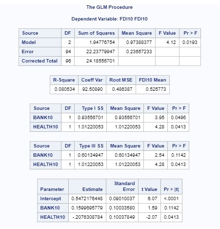
The variables I used in the regression are (in form of panel data: if they grow from year 2012 to 2013 a number 1 is given, if they fall or stay the same a 0 is given):
FDI: FOREIGN DIRECT INVESTMENT
BANK: COMERCIAL BANK BRANCHES
HEALTH: OUT-OF-POCKET HEALTH EXPENDITURE
Unfortunately, this week has been very hectic for me at work and did not have time to write that much in here. However, I will the pictures of what I have so far and my writing so far, and continue working on my research paper more in depth this week:
An approach for predicting foreign direct investment of a country from other well-being and economic variables.
This is my final paper for the course Data Analysis and Interpretation, from Wesleyan University. The report analyses the World Bank data set in order to select alternative variables to predict a country’s foreign direct investment. This is helpful to make decisions on which areas to improve development to increase citizens’ standard of living and economy growth.
The purpose of this study is to identify the best predictors of foreign direct investment in a country from multiple well-being and economic indicators such as number of secured internet serves and number of internet users, fixed broadband subscriptions, out-of-pocket health expenditures, private credit bureau, consumption of fixed capital, inflation, and commercial bank branches.
As an economist and consultant, I use these variables daily to analyze and respond clients’ questions on the associations of these variables and how they can affect foreign direct investment in their country. Having a clearer idea of how FDI can be affected by other factors will be useful information for me to understand and use in my work.
The result of the research could be used to focus on indicators that could attract more foreign investment, and as a result help the country’s economy grow and improve standard of living. FDI is an economic indicator that can represent how well a country is doing and how attractive its economy is to others. The more attractive a country’s economy is, the bigger the chance to grow and develop. This research could help to identify the relation this economic indicator has with other variables that usually are not always associated with FDI.
The sample included N=248 countries for the years 2012 and 2013. All variables have data observations for a minimum of 190 countries.
For all the variables, I calculated the percentage variation of years 2012 and 2013. Therefore, the variables are used in percentage form and tell us how much the variable grew or fell from year 2012 to year 2013. If the number is positive, it means that the variable grew from 2012 to 2013. If it is negative, the variable fell.
All variables are calculated with this measurement, but they also have different attributes. The dependent variable foreign direct investment is measured as percentage of GDP. For some predictors: fixed broadband subscriptions is measured per 100 people,out-of-pocket health expenditure as percentage of total expenditure on health, private credit bureau coverage as percentage of adults, secure internet servers per 1 million people, adjusted savings: consumption of fixed capital as percentage of GNI inflation as annual percentage, commercial bank branches per 100,000 adults, and number of internet users per 100 people.
Analyses
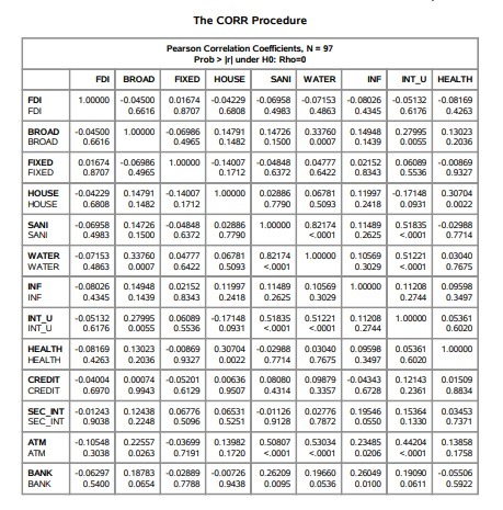
Since my variables are all quantitative, the distribution for the predictors and the response variable were evaluated by calculating pearson correlation and scatter plots were also used to examine the associations between foreign direct investment of a country and the independent variables.
Lasso regression was used identify the variables that best predict the increase or decrease of foreign direct investment in a country. The model was estimated on a training data set with a random sample of 60% of the batches (N=32). There are some tests left to do, however so far it is evident that the increase or decrease of foreign direct investment is explained by the movement of inflation and secured internet servers, which are a representation of how well and how developed a country is.
0 notes
Text
Capstone week 2
An approach for predicting foreign direct investment of a country from other well-being and economic variables.
This is my final paper for the course Data Analysis and Interpretation, from Wesleyan University. The report analyses the World Bank data set in order to select alternative variables to predict a country’s foreign direct investment. This is helpful to make decisions on which areas to improve development to increase citizens’ standard of living and economy growth.
The purpose of this study is to identify the best predictors of foreign direct investment in a country from multiple well-being and economic indicators such as number of secured internet serves and number of internet users, fixed broadband subscriptions, out-of-pocket health expenditures, private credit bureau, consumption of fixed capital, inflation, and commercial bank branches.
As an economist and consultant, I use these variables daily to analyze and respond clients’ questions on the associations of these variables and how they can affect foreign direct investment in their country. Having a clearer idea of how FDI can be affected by other factors will be useful information for me to understand and use in my work.
The result of the research could be used to focus on indicators that could attract more foreign investment, and as a result help the country’s economy grow and improve standard of living. FDI is an economic indicator that can represent how well a country is doing and how attractive its economy is to others. The more attractive a country’s economy is, the bigger the chance to grow and develop. This research could help to identify the relation this economic indicator has with other variables that usually are not always associated with FDI.
Sample
The sample included N=248 countries for the years 2012 and 2013. All variables have data observations for a minimum of 190 countries.
Measures
For all the variables, I calculated the percentage variation of years 2012 and 2013. Therefore, the variables are used in percentage form and tell us how much the variable grew or fell from year 2012 to year 2013. If the number is positive, it means that the variable grew from 2012 to 2013. If it is negative, the variable fell.
All variables are calculated with this measurement, but they also have different attributes. The dependent variable foreign direct investment is measured as percentage of GDP. For some predictors: fixed broadband subscriptions is measured per 100 people,out-of-pocket health expenditure as percentage of total expenditure on health, private credit bureau coverage as percentage of adults, secure internet servers per 1 million people, adjusted savings: consumption of fixed capital as percentage of GNI inflation as annual percentage, commercial bank branches per 100,000 adults, and number of internet users per 100 people.
Analyses
Since my variables are all quantitative, the distribution for the predictors and the response variable were evaluated by calculating pearson correlation and scatter plots were also used to examine the associations between foreign direct investment of a country and the independent variables.
Lasso regression was used identify the variables that best predict the increase or decrease of foreign direct investment in a country. The model was estimated on a training data set with a random sample of 60% of the batches (N=32). There are some tests left to do, however so far it is evident that the increase or decrease of foreign direct investment is explained by the movement of inflation and secured internet servers, which are a representation of how well and how developed a country is.
0 notes
Text
Research title and explanation
Title
Foreign direct investment is associated with well-being economic indicators of a country, such as number of internet users, access to electricity, and improved sanitation facilities.
Introduction to research question
The purpose of this study is to identify the best predictors of foreign direct investment in a country from multiple well-being economic indicators such as number of internet users, access to electricity, and improved sanitation facilities.
As an economist and consultant, I use these variables daily to analyze and respond clients’ questions on the associations of these variables and how they can affect foreign direct investment in their country. Having a clearer idea of how FDI can be affected by other factors will be useful information for me to understand and use in my work.
FDI is an economic indicator that can represent how well a country is doing and how attractive its economy is to others. The more attractive a country’s economy is, the bigger the chance to grow and develop. This research could help to identify the relation this economic indicator has with other variables that usually are not always associated with FDI.
0 notes
Text
Course 4 - Week 4
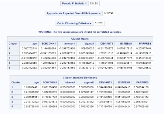


For cluster one, we can see there is a higher correlation between gpa and cigarette availability.
For the second cluster, the highest correlation is with inhever1.
In cluster four, they were more likely to have parents presence in their lives (low correlation).
In cluster two, the adolescents were less likely to have cigarette availability.
Adolescents in cluster 2 had the higher gpa, which were the ones that had lowest likelihood to have cigarette availability.
CODE:
LIBNAME mydata "/courses/d1406ae5ba27fe300" access=readonly;
DATA clust;
set mydata.treeaddhealth;
idnum=_n_;
keep age schconn1 inhever1 cigavail
deviant1 esteem1 parpres gpa1;
if cmiss (of _all_) then delete;
run;
ods graphics on;
proc surveyselect data=clust out=traintest seed=123
samprate=0.7 method=srs outall;
run;
data clus_train;
set traintest;
if selected=1;
run;
data clust_test;
set traintest;
if selected=0;
run;
proc standard data=clus_train out=clustvar mean=0 std=1;
var age schconn1 inhever1 cigavail
deviant1 esteem1 parpres;
run;
%macro kmean(K);
proc fastclus data=clustvar out=outdata&K. outstat=cluststat&K.
maxclusters= &K. maxiter=300;
var age schconn1 inhever1 cigavail
deviant1 esteem1 parpres;
run;
%mend;
%kmean (1);
%kmean (2);
%kmean (3);
%kmean (4);
%kmean (5);
data clus1;
set cluststat1;
nclust=1;
if_type_='RSQ';
keep nclust over_all;
run;
data clus2;
set cluststat2;
nclust=2;
if_type_='RSQ';
keep nclust over_all;
run;
data clus3;
set cluststat3;
nclust=3;
if_type_='RSQ';
keep nclust over_all;
run;
data clus4;
set cluststat4;
nclust=4;
if_type_='RSQ';
keep nclust over_all;
run;
data clus5;
set cluststat5;
nclust=5;
if_type_='RSQ';
keep nclust over_all;
run;
data clusrsquare;
set clus1 clus2 clus3 clus4 clus5;
run;
proc gplot data=clusrsquare;
plot over_all*nclust;
run;
proc candisc data=outdata4 out=clustcan;
class cluster;
var age schconn1 inhever1 cigavail
deviant1 esteem1 parpres;
run;
proc sgplot data=clustcan;
scatter y=can2 x=can1 / group=cluster;
run;
data gpa_data;
set clus_train;
keep age gpa1;
run;
proc sort data=outdata4;
by age;
run;
proc sort data=gpa_data;
by age;
run;
data merged;
merge outdata4 gpa_data;
by age;
run;
proc sort data=merged;
var gpa1;
by cluster;
run;
proc anova data=merged;
class cluster;
model gpa1 = cluster;
means cluster/tukey;
run;
0 notes
Text
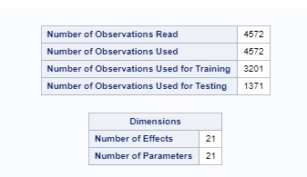
Course 4 - Week 3
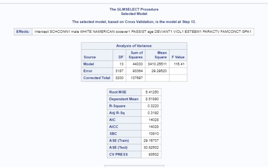
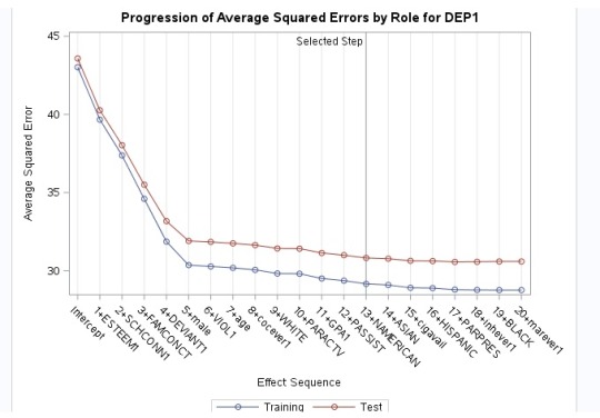
The dependent variables is dep1 (depression).
According to the LASSO Regression results, it looks like the most important predictor of depression is self esteem followed by school connectiveness. The model selected as the best model (with lowest sum of residual sum of squares) is at the predictor native american.
In the plot of the change in the regression coefficient: esteem1, school connectiveness and family connectiveness had the largest regression coefficient. Those three predictors are negatively associated with depression.
The CV PRESS plot shows how the model decreases rapidly until a point were adding more predictors does not lead to much production in the residual sum of squares.
CODE:
LIBNAME mydata "/courses/d1406ae5ba27fe300" access=readonly;
DATA new;
set mydata.treeaddhealth;
if bio_sex=1 then male=1;
if bio_sex=2 then male=0;
if cmiss(of _all_) then delete;
run;
ods graphics on;
proc surveyselect data=new out=traintest seed=120
samprate=0.7 method=srs outall;
run;
proc glmselect data=traintest plots=all seed=120;
partition ROLE=selected(train='1' test='0');
model dep1= schconn1 male hispanic white black namerican asian marever1 cocever1
inhever1 cigavail passist age deviant1 viol1 esteem1 parpres paractv
famconct gpa1/selection=lar(choose=cv stop=none) cvmethod=random(10);
run;


0 notes
Photo
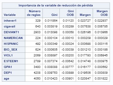
COURSE 4 - WEEK 2
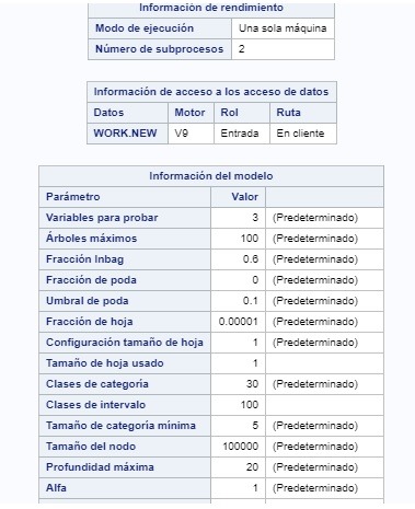
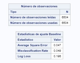
For this assignment, I used caterogical variables for the first input statement: race, gender, cigarette availability, and more.
For the quantitative variables I used: violence, self esteem, depression, GPA, and more.
The most important one for explaining cocaine inherence proved to be cigarette availability and inherence of substances.
code:
LIBNAME mydata "/courses/d1406ae5ba27fe300" access=readonly;
DATA new; set mydata.treeaddhealth;
PROC SORT; BY AID;
PROC HPFOREST;
target cocever1/level=nominal;
input HISPANIC BIO_SEX inhever1 cigavail namerican /level=nominal;
input age DEVIANT1 VIOL1 ESTEEM1 GPA1 DEP1 /level=interval;
RUN;
0 notes
Photo


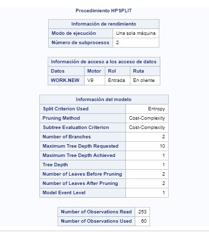
COURSE 4 - WEEK 1
I struggled with this assignment, because I could not figure out how to create the decision tree. However, this is what I got:
The decision tree was made to test nonlinear relationships among series of explanatory and a categorical response variables. The response variables is the amount of breast cancer cases per 100th people. The following explanatory variables were included as possible contributors to evaluating the probability of breast cancer cases: income per person, female employment rate, alcohol consumption, life expectancy, urban rate, electricity per person, suicide rate per 100th and oil per person in countries.
The electicity per person is the first division. After doing the pruning, the tree was left with 2 leaves.
CODE:
LIBNAME mydata "/courses/d1406ae5ba27fe300" access=readonly;
DATA new; set mydata.gapminder;
/*data management for breastcancerper100TH*/
IF breastcancerper100TH>=3.9 AND breastcancerper100TH<34.4 THEN breastcancerper100th=1;
ELSE IF breastcancerper100TH>=34.4 AND breastcancerper100TH<102 THEN breastcancerper100th=2;
ods graphics on;
proc hpsplit seed=10000;
class breastcancerper100th incomeperperson femaleemployrate alcconsumption
lifeexpectancy urbanrate relectricperperson suicideper100th oilperperson;
model breastcancerper100th = incomeperperson femaleemployrate alcconsumption
lifeexpectancy urbanrate relectricperperson suicideper100th oilperperson;
grow entropy;
prune costcomplexity;
RUN;
0 notes
Photo


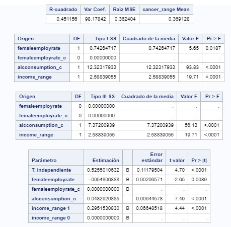
COURSE 3 - WEEK 4
In the After adjusting for potential confounding factors (alcohol consumption, 1 being those with higher consumption, and income per person), the odds of having breast cancer cases are for higher alcohol consumption (OR=12.465 95% CI=5.035-30.860 p-value=<0.0001). For higher income was was laso significant, (OR=7.481 CI=3.024-18.509 p-value=<0.0001). However, countries that have higher consumption have higher chance to have more breast cancer cases.
CODE:
LIBNAME mydata "/courses/d1406ae5ba27fe300" access=readonly;
DATA new; set mydata.gapminder (KEEP= country incomeperperson breastcancerper100th
femaleemployrate alcconsumption);
IF MISSING(incomeperperson) OR MISSING(breastcancerper100TH)
OR MISSING(femaleemployrate) OR MISSING(alcconsumption) THEN DELETE;
LABEL income_range="Income per Person Range from Lowest=1 to Highest=5"
cancer_range="Breast Cancer Cases Range Lowest=1 to Highest=5"
employ_range="Female Employees 15+ (% population) Range Lowest=1 to Highest=5"
alcconsumption_range="Alcohol consumption per adult 15+ Range" ;
/*data management for incomeperperson*/
IF incomeperperson>=103 AND incomeperperson<3174.23 THEN income_range=0;
ELSE IF incomeperperson>=3174.23 AND incomeperperson<27111.7 THEN income_range=1;
/*data management for breastcancerper100TH*/
IF breastcancerper100TH>=3.9 AND breastcancerper100TH<34.4 THEN cancer_range=0;
ELSE IF breastcancerper100TH>=34.4 AND breastcancerper100TH<102 THEN cancer_range=1;
/*data management for femaleemployrate*/
IF femaleemployrate>=12.4 AND femaleemployrate<53.8 THEN employ_range=0;
ELSE IF femaleemployrate>=53.8 AND femaleemployrate<83.3 THEN employ_range=1;
/*data management for alcconsumption*/
IF alcconsumption>=0.1 AND alcconsumption<7.6 THEN alcconsumption_range=0;
ELSE IF alcconsumption>=7.6 AND alcconsumption<23.1 THEN alcconsumption_range=1;
RUN;
****************************************************************************************************
CATEGORICAL EXPLANATORY VARIABLES RE-VISITED (3+ CATEGORIES)
****************************************************************************************************;
* centering quantitative number of some explanatory variables later regression;
* print mean;
PROC MEANS;
var femaleemployrate alcconsumption;
run;
* centering (subtract mean);
data new2;
set new;
femaleemployrate_c = femaleemployrate - 47.9596272;
alcconsumption_c = alcconsumption - 6.8501242;
run;
* check coding;
PROC MEANS;
var femaleemployrate_c alcconsumption_c;
run;
*adding variable, reference group lowest income countries;
PROC GLM;
class income_range (ref="0");
model cancer_range=femaleemployrate femaleemployrate_c alcconsumption_c
income_range/solution;
run;
*adding variable, reference group hieghest income countries;
PROC GLM;
class income_range (ref="1");
model cancer_range=femaleemployrate
income_range/solution;
run;
****************************************************************************************************
LOGISTIC REGRESSION
****************************************************************************************************;
Proc logistic descending; model cancer_range=alcconsumption_range income_range;
run;
0 notes
Photo
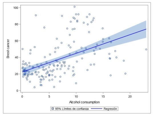
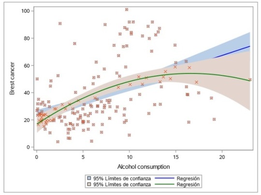


COURSE 3 - WEEK 3
My results did not support my hypothesis that more alcohol consumption and female employment increase the probability of having more breast cancer cases.
In the model we can see that alcconsumption_c, alcconsumption^2, and femaleemployrate_c are not significant. The p-value for the first to is less than 0.05 but femaleemployrate has a p-value greater, which suggests that the variable is not significant in this relationship. However, for the two variables that are significant the betas are very small: one more value for Alcconsumption_c suggests that it will increase the breast cancer cases by 0.00305673.
What I did notice is that after I added the confounding variables, the R-squared increased to around 59%. Meaning that 59% of the variance in the response variables (breastcancerper100th) is explained by the variance in the explanatory variables. However, this is not acceptable because the betas are too low.
In the residual plot graphs for all the variables, shows they are mainly scatterplots without linear relationship, residuals are spread out in a random pattern.
In the residual graph we can see that the fit of this model is poor (outliers).
CODE:
LIBNAME mydata "/courses/d1406ae5ba27fe300" access=readonly;
data new; set mydata.gapminder;
run;
* scatterplot with linear regression line femaleemployrate response variable;
proc sgplot;
reg x=alcconsumption y=breastcancerper100TH / lineattrs=(color=blue thickness=2) clm;
yaxis label="Brest cancer";
xaxis label="Alcohol consumption";
run;
* scatterplot with linear and quadratic regression line;
proc sgplot;
reg x=alcconsumption y=breastcancerper100TH / lineattrs=(color=blue thickness=2) degree=1 clm;
reg x=alcconsumption y=breastcancerper100TH / lineattrs=(color=green thickness=2) degree=2 clm;
yaxis label="Brest cancer";
xaxis label="Alcohol consumption";
run;
* centering quantitative explanatory variables;
data new2; set new;
if alcconsumption ne . and breastcancerper100TH ne . and femaleemployrate ne .;
alcconsumption_c=incomeperperson-6.8501242;
femaleemployrate_c=femaleemployrate-47.9596272;
run;
proc means; var alcconsumption femaleemployrate;
run;
* check coding;
proc means; var alcconsumption_c femaleemployrate_c;
run;
* linear regression model;
PROC glm;
model breastcancerper100TH=alcconsumption_c/solution clparm;
run;
* polynomial regression model;
PROC glm;
model breastcancerper100TH=alcconsumption_c alcconsumption_c*alcconsumption_c/solution clparm;
run;
*************************************************************************************************
EVALUATING MODEL FIT
*************************************************************************************************;
* multiple regression adding internet use rate;
PROC glm;
model breastcancerper100TH=alcconsumption_c alcconsumption_c*alcconsumption_c femaleemployrate_c/solution clparm;
run;
* request regression diagnostic plots;
PROC glm PLOTS(unpack)=all;
model breastcancerper100TH=alcconsumption_c alcconsumption_c*alcconsumption_c
femaleemployrate_c/solution clparm;
output residual=res student=stdres out=results;
run;
* plot of standardized residuals for each observation;
proc gplot;
label stdres="Standardized Residual" country="Country";
plot stdres*country/vref=0;
run;
* using proc reg to get a partial regression plot;
* calculate quadratic terms;
data partial;
set new2;
alcconsumption2=alcconsumption_c*alcconsumption_c;
run;
*partial regression plot;
PROC reg plots=partial;
model breastcancerper100TH=alcconsumption alcconsumption2
femaleemployrate/partial;
run;
0 notes


Text
Course 3 - Week 2
As it is clear, there is not a strong relationship between these variables. Even though R-square is 53% (which means that the variation in income per person explains 53% of the variation in breast cancer cases) and the p-value are lower than 0.05, and increase in income only increases the breast cancer cases by 0.002. This is a small impact in the dependent variable.
The regression: breastcancerper100th = 26.03 + 0.002 * incomeperperson
Also, the scatterplot shows this model has outliers, which affects our analysis.
CODE:
LIBNAME mydata "/courses/d1406ae5ba27fe300" access=readonly;
DATA new; set mydata.gapminder (KEEP= country incomeperperson breastcancerper100th
femaleemployrate alcconsumption);
IF MISSING(incomeperperson) OR MISSING(breastcancerper100TH)
OR MISSING(femaleemployrate) OR MISSING(alcconsumption) THEN DELETE;
LABEL income_range="Income per Person Range from Lowest=1 to Highest=5"
cancer_range="Breast Cancer Cases Range Lowest=1 to Highest=5"
employ_range="Female Employees 15+ (% population) Range Lowest=1 to Highest=5"
alcconsumption_range="Alcohol consumption per adult 15+ Range" ; PROC SORT; by country;
PROC sgplot;
reg x=incomeperperson y=breastcancerper100th / lineattrs=(color=blue thickness=2);
title "Scatterplot for the Association Between breast cancer and income";
yaxis label="Income per person";
xaxis label="Breast cancer cases";
run;
title;* basic linear regression;
PROC glm;
model breastcancerper100th=incomeperperson/solution;
run;
0 notes
Text
Course 3 - Week 1
The sample is composed by data extracted from every country, and from different locations (I could not find the exact place, like a hospital, from where the sample was drawn from). Since this is data of all the countries, is hard to explain the sample, because every country has different ethnic majority. For the purpose of the analysis, I divided the variables in quintiles, so that, for example, the income groups are divided in order and with similar income. With this strategy, for example, I have been able to find the relationship between breast cancer cases and income per person is that the higher the income, the higher the number of breast cancer cases.
Random sampling was used to gather this data. GapMinder collects data from a handful of sources (example: United Nations Statistics Division). It includes data from 195 UN members, aggregating data for Serbia and Montenegro. In addition, it includes data for 24 other areas, generating a total of 215 areas.
The measure of breast cancer cases was drawn from country level data compiled by ARC (International Agency for Research on Cancer). It measures the number of new cases of breast cancer in 100,000 female residents in each country during 2002. The measure of income per person was drawn from country level data compiled by the World Bank Work Development Indicators, and measures the 2010 Gross Domestic Product per capita in constant 2000 US$ in every country. The variable for female employ rate is from 2007, and the participants are female employees age 15+ (% of population) employed in the given year. For the current analysis, the variables were each binned into five categories based on a quintile split.
0 notes
Text
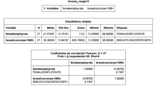
Course 2 - Week 4
We can see that the correlation for the variables for breast cancer cases and female employment rate is significant for countries in the range 2 (the next range after the one for lowest income countries) and range 5 (range for highest income countries).
For range 2: the correlation between female employ rate and breast cancer cases is negative in this range of countries (second after the poorest).
For range 5: the correlation between the two variables is positive, but not very strong, in the wealthiest countries.
CODE:
LIBNAME mydata "/courses/d1406ae5ba27fe300" access=readonly;
DATA new; set mydata.gapminder (KEEP= country incomeperperson breastcancerper100th
femaleemployrate alcconsumption);
IF MISSING(incomeperperson) OR MISSING(breastcancerper100TH)
OR MISSING(femaleemployrate) OR MISSING(alcconsumption) THEN DELETE;
/*data management for incomeperperson*/
IF incomeperperson>=103 AND incomeperperson<546.656 THEN income_range=1;
ELSE IF incomeperperson>=546.656 AND incomeperperson<1533.05 THEN income_range=2;
ELSE IF incomeperperson>=1533.05 AND incomeperperson<3174.23 THEN income_range=3;
ELSE IF incomeperperson>=3174.23 AND incomeperperson<8580.4 THEN income_range=4;
ELSE IF incomeperperson>=8580.4 AND incomeperperson<27111.7 THEN income_range=5;
RUN;
PROC SORT; by COUNTRY;
PROC SORT; by income_range;
PROC CORR; VAR femaleemployrate breastcancerper100TH; BY income_range;
RUN;


0 notes
Text
Course 2 - Week 3
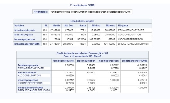
In this assignment, we can see the correlation of my quantitative independent variables (femaleemployrate, alcconsumption and incomeperperson) and my quantitative dependent variable (breastcancerper100th). In the table for Pearson Correlation, the strongest correlation is between breastcancerper100th and incomeperperson: 0.73. This is a strong positive correlation, which means that the higher the income the higher the number of breast cancer cases. If we do r square, we find that the income can explain 53% of the variation in breast cancer cases. There is a chance this correlation is given because higher income people have better chances of detecting the cancer, than lower income people, due to the facility of paying for tests and keeping a continuity of the disease. For the case of alcohol consumption, the correlation with breast cancer cases is positive but it is not very strong, r square is 23% (only explains 23% of the variation in breast cancer cases).
LIBNAME mydata "/courses/d1406ae5ba27fe300" access=readonly;
DATA new; set mydata.gapminder (KEEP= country incomeperperson breastcancerper100th
femaleemployrate alcconsumption);
IF MISSING(incomeperperson) OR MISSING(breastcancerper100TH)
OR MISSING(femaleemployrate) OR MISSING(alcconsumption) THEN DELETE;
LABEL income_range="Income per Person Range from Lowest=1 to Highest=5"
cancer_range="Breast Cancer Cases Range Lowest=1 to Highest=5"
employ_range="Female Employees 15+ (% population) Range Lowest=1 to Highest=5"
alcconsumption_range="Alcohol consumption per adult 15+ Range" ;
/*data management for incomeperperson*/
IF incomeperperson>=103 AND incomeperperson<546.656 THEN income_range=1;
ELSE IF incomeperperson>=546.656 AND incomeperperson<1533.05 THEN income_range=2;
ELSE IF incomeperperson>=1533.05 AND incomeperperson<3174.23 THEN income_range=3;
ELSE IF incomeperperson>=3174.23 AND incomeperperson<8580.4 THEN income_range=4;
ELSE IF incomeperperson>=8580.4 AND incomeperperson<27111.7 THEN income_range=5;
/*data management for breastcancerper100TH*/
IF breastcancerper100TH>=3.9 AND breastcancerper100TH<19.1 THEN cancer_range=1;
ELSE IF breastcancerper100TH>=19.1 AND breastcancerper100TH<25.9 THEN cancer_range=2;
ELSE IF breastcancerper100TH>=25.9 AND breastcancerper100TH<34.4 THEN cancer_range=3;
ELSE IF breastcancerper100TH>=34.4 AND breastcancerper100TH<54.4 THEN cancer_range=4;
ELSE IF breastcancerper100TH>=54.4 AND breastcancerper100TH<102 THEN cancer_range=5;
/*data management for femaleemployrate*/
IF femaleemployrate>=12.4 AND femaleemployrate<40.5 THEN employ_range=1;
ELSE IF femaleemployrate>=40.5 AND femaleemployrate<48.6 THEN employ_range=2;
ELSE IF femaleemployrate>=48.6 AND femaleemployrate<53.8 THEN employ_range=3;
ELSE IF femaleemployrate>=53.8 AND femaleemployrate<65 THEN employ_range=4;
ELSE IF femaleemployrate>=65 AND femaleemployrate<83.3 THEN employ_range=5;
/*data management for alcconsumption*/
IF alcconsumption>=0.1 AND alcconsumption<1.9 THEN alcconsumption_range=1;
ELSE IF alcconsumption>=1.9 AND alcconsumption<5.0 THEN alcconsumption_range=2;
ELSE IF alcconsumption>=5.0 AND alcconsumption<7.6 THEN alcconsumption_range=3;
ELSE IF alcconsumption>=7.6 AND alcconsumption<11.3 THEN alcconsumption_range=4;
ELSE IF alcconsumption>=11.3 AND alcconsumption<23.1 THEN alcconsumption_range=5;
RUN;
PROC SORT; by country;
PROC CORR; VAR femaleemployrate alcconsumption incomeperperson breastcancerper100TH;
RUN;
0 notes
Text
COURSE 2 - WEEK 2
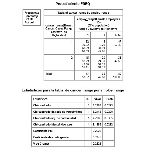


Course 2 - Week 2
My hypothesis, and database selected, consist on using quantitative variables. However, for this assignment, I categorized the variables.
To avoid Type I error:
I used the Bonferroni Adjustment.
Comparisons: 9
0.05/10 = 0.005
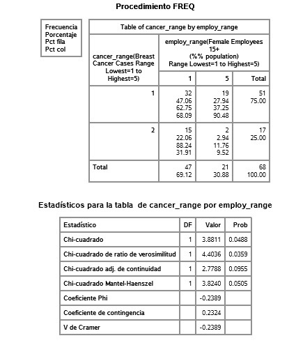
For the table comparing employ_range 2 and 5: they are significantly different (p=0.0004), reject null hypothesis. Breast cancer cases is significantly different to female employment rate in countries between range 2 and 5.
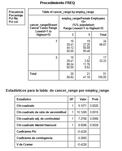
The same goes for comparing employ_range 3 and 5 (p=0.0025).
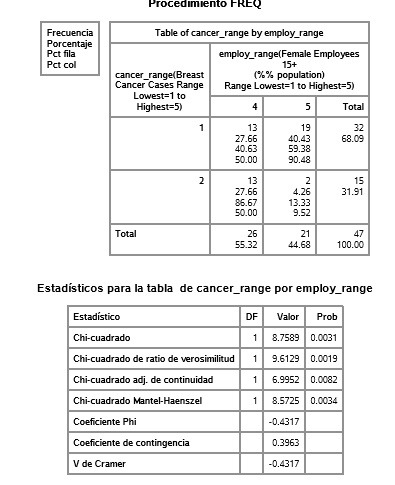
The rest seem not to be significantly different to each other.
CODE:
LIBNAME mydata "/courses/d1406ae5ba27fe300" access=readonly;
DATA new; set mydata.gapminder (KEEP= country incomeperperson breastcancerper100th
femaleemployrate alcconsumption);
IF MISSING(incomeperperson) OR MISSING(breastcancerper100TH)
OR MISSING(femaleemployrate) OR MISSING(alcconsumption) THEN DELETE;
LABEL income_range="Income per Person Range from Lowest=1 to Highest=5"
cancer_range="Breast Cancer Cases Range Lowest=1 to Highest=5"
employ_range="Female Employees 15+ (% population) Range Lowest=1 to Highest=5"
alcconsumption_range="Alcohol consumption per adult 15+ Range" ;
/*data management for incomeperperson*/
IF incomeperperson>=103 AND incomeperperson<546.656 THEN income_range=1;
ELSE IF incomeperperson>=546.656 AND incomeperperson<1533.05 THEN income_range=2;
ELSE IF incomeperperson>=1533.05 AND incomeperperson<3174.23 THEN income_range=3;
ELSE IF incomeperperson>=3174.23 AND incomeperperson<8580.4 THEN income_range=4;
ELSE IF incomeperperson>=8580.4 AND incomeperperson<27111.7 THEN income_range=5;
/*data management for breastcancerper100TH*/
IF breastcancerper100TH>=3.9 AND breastcancerper100TH<34.4 THEN cancer_range=1;
ELSE IF breastcancerper100TH>=34.4 AND breastcancerper100TH<102 THEN cancer_range=2;
/*data management for femaleemployrate*/
IF femaleemployrate>=12.4 AND femaleemployrate<40.5 THEN employ_range=1;
ELSE IF femaleemployrate>=40.5 AND femaleemployrate<48.6 THEN employ_range=2;
ELSE IF femaleemployrate>=48.6 AND femaleemployrate<53.8 THEN employ_range=3;
ELSE IF femaleemployrate>=53.8 AND femaleemployrate<65 THEN employ_range=4;
ELSE IF femaleemployrate>=65 AND femaleemployrate<83.3 THEN employ_range=5;
/*data management for alcconsumption*/
IF alcconsumption>=0.1 AND alcconsumption<1.9 THEN alcconsumption_range=1;
ELSE IF alcconsumption>=1.9 AND alcconsumption<5.0 THEN alcconsumption_range=2;
ELSE IF alcconsumption>=5.0 AND alcconsumption<7.6 THEN alcconsumption_range=3;
ELSE IF alcconsumption>=7.6 AND alcconsumption<11.3 THEN alcconsumption_range=4;
ELSE IF alcconsumption>=11.3 AND alcconsumption<23.1 THEN alcconsumption_range=5;
RUN;
PROC SORT; by country;
/*PROC ANOVA; CLASS income_range;
MODEL breastcancerper100TH=income_range;
MEANS income_range/DUNCAN;
PROC ANOVA; CLASS employ_range;
MODEL breastcancerper100TH=employ_range;
MEANS employ_range/DUNCAN;
PROC ANOVA; CLASS alcconsumption_range;
MODEL breastcancerper100TH=alcconsumption_range;
MEANS alcconsumption_range/DUNCAN;
RUN;*/
PROC FREQ; TABLES cancer_range*employ_range/CHISQ;
RUN;
DATA COMPARISON1; SET NEW;
IF employ_range=1 OR employ_range=2;
PROC SORT; BY COUNTRY;
PROC FREQ; TABLES cancer_range*employ_range/CHISQ;
RUN;
DATA COMPARISON2; SET NEW;
IF employ_range=1 OR employ_range=3;
PROC SORT; BY COUNTRY;
PROC FREQ; TABLES cancer_range*employ_range/CHISQ;
RUN;
DATA COMPARISON3; SET NEW;
IF employ_range=1 OR employ_range=4;
PROC SORT; BY COUNTRY;
PROC FREQ; TABLES cancer_range*employ_range/CHISQ;
RUN;
DATA COMPARISON4; SET NEW;
IF employ_range=1 OR employ_range=5;
PROC SORT; BY COUNTRY;
PROC FREQ; TABLES cancer_range*employ_range/CHISQ;
RUN;
DATA COMPARISON5; SET NEW;
IF employ_range=2 OR employ_range=3;
PROC SORT; BY COUNTRY;
PROC FREQ; TABLES cancer_range*employ_range/CHISQ;
RUN;
DATA COMPARISON6; SET NEW;
IF employ_range=2 OR employ_range=4;
PROC SORT; BY COUNTRY;
PROC FREQ; TABLES cancer_range*employ_range/CHISQ;
RUN;
DATA COMPARISON7; SET NEW;
IF employ_range=2 OR employ_range=5;
PROC SORT; BY COUNTRY;
PROC FREQ; TABLES cancer_range*employ_range/CHISQ;
RUN;
DATA COMPARISON8; SET NEW;
IF employ_range=3 OR employ_range=4;
PROC SORT; BY COUNTRY;
PROC FREQ; TABLES cancer_range*employ_range/CHISQ;
RUN;
DATA COMPARISON9; SET NEW;
IF employ_range=3 OR employ_range=5;
PROC SORT; BY COUNTRY;
PROC FREQ; TABLES cancer_range*employ_range/CHISQ;
RUN;
DATA COMPARISON10; SET NEW;
IF employ_range=4 OR employ_range=5;
PROC SORT; BY COUNTRY;
PROC FREQ; TABLES cancer_range*employ_range/CHISQ;
RUN;
0 notes
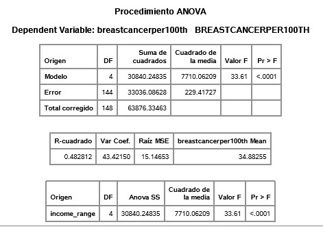
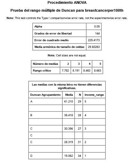
Photo


COURSE 2 - WEEK 1
Null Hypothesis: There is NO relationship between dependent variable breast cancer cases and independent variables alcohol consumption, income per person and female employment rate.
Alternative Hypothesis: There is a relationship between dependent variable breast cancer cases and independent variables alcohol consumption, income per person and female employment rate.
I had to pass the independet variables from quantitative to categorical to be able to do the ANOVA test.
- As seen in the tables, all three independet variables have a p-value lower than 0.05, which means there IS an association between breast cancer and these three independet variables.
- All we know is that not all means are equal in each independent categorical variable group. This is why the next step is to do a POST HOC TEST to prevent the Type 1 error.
Duncan tables:
- For indp. var. income_range: group 3 is sig. different to 1,4 and 5. Group 5 to 4, 3, 2, 1. and so on.
income_range group 5, highest income (wealthiest countries), has significantly more cases of breast cancer than group 1, 2, 3, and 4.
- For indp. var. employ_range: group 4 is significantly different than groups 1 and 5. Group 2 is sig. different to groups 1 and 5. Group 3 is sig. different to group 5. Group 1 to 4, 2 and 5. Group 5 to 1, 2, 3, 4.
employ_range group 5, countries with highest female employment rate, has significantly more breast cancer cases than groups 1, 2, 3, and 4.
- For indp. var. alcconsumption_range: 5 and 4 are not sig. different, as well as 3, 2, and 1.
alcconsumption_range group 5, countries with highest alcohol consumption, does not has significantly more breast cancer cases than group 4, but is does for groups 1, 2, and 3.
The code used for this assignment:
LIBNAME mydata "/courses/d1406ae5ba27fe300" access=readonly;
DATA new; set mydata.gapminder (KEEP= country incomeperperson breastcancerper100th
femaleemployrate alcconsumption);
IF MISSING(incomeperperson) OR MISSING(breastcancerper100TH)
OR MISSING(femaleemployrate) OR MISSING(alcconsumption) THEN DELETE;
LABEL income_range="Income per Person Range from Lowest=1 to Highest=5"
cancer_range="Breast Cancer Cases Range Lowest=1 to Highest=5"
employ_range="Female Employees 15+ (% population) Range Lowest=1 to Highest=5"
alcconsumption_range="Alcohol consumption per adult 15+ Range" ;
/*data management for incomeperperson*/
IF incomeperperson>=103 AND incomeperperson<546.656 THEN income_range=1;
ELSE IF incomeperperson>=546.656 AND incomeperperson<1533.05 THEN income_range=2;
ELSE IF incomeperperson>=1533.05 AND incomeperperson<3174.23 THEN income_range=3;
ELSE IF incomeperperson>=3174.23 AND incomeperperson<8580.4 THEN income_range=4;
ELSE IF incomeperperson>=8580.4 AND incomeperperson<27111.7 THEN income_range=5;
/*data management for breastcancerper100TH*/
IF breastcancerper100TH>=3.9 AND breastcancerper100TH<19.1 THEN cancer_range=1;
ELSE IF breastcancerper100TH>=19.1 AND breastcancerper100TH<25.9 THEN cancer_range=2;
ELSE IF breastcancerper100TH>=25.9 AND breastcancerper100TH<34.4 THEN cancer_range=3;
ELSE IF breastcancerper100TH>=34.4 AND breastcancerper100TH<54.4 THEN cancer_range=4;
ELSE IF breastcancerper100TH>=54.4 AND breastcancerper100TH<102 THEN cancer_range=5;
/*data management for femaleemployrate*/
IF femaleemployrate>=12.4 AND femaleemployrate<40.5 THEN employ_range=1;
ELSE IF femaleemployrate>=40.5 AND femaleemployrate<48.6 THEN employ_range=2;
ELSE IF femaleemployrate>=48.6 AND femaleemployrate<53.8 THEN employ_range=3;
ELSE IF femaleemployrate>=53.8 AND femaleemployrate<65 THEN employ_range=4;
ELSE IF femaleemployrate>=65 AND femaleemployrate<83.3 THEN employ_range=5;
/*data management for alcconsumption*/
IF alcconsumption>=0.1 AND alcconsumption<1.9 THEN alcconsumption_range=1;
ELSE IF alcconsumption>=1.9 AND alcconsumption<5.0 THEN alcconsumption_range=2;
ELSE IF alcconsumption>=5.0 AND alcconsumption<7.6 THEN alcconsumption_range=3;
ELSE IF alcconsumption>=7.6 AND alcconsumption<11.3 THEN alcconsumption_range=4;
ELSE IF alcconsumption>=11.3 AND alcconsumption<23.1 THEN alcconsumption_range=5;
RUN;
PROC SORT; by country;
PROC ANOVA; CLASS income_range;
MODEL breastcancerper100TH=income_range;
MEANS income_range/DUNCAN;
PROC ANOVA; CLASS employ_range;
MODEL breastcancerper100TH=employ_range;
MEANS employ_range/DUNCAN;
PROC ANOVA; CLASS alcconsumption_range;
MODEL breastcancerper100TH=alcconsumption_range;
MEANS alcconsumption_range/DUNCAN;
RUN;
0 notes


