Results

Descriptive Statistics

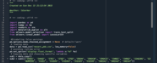
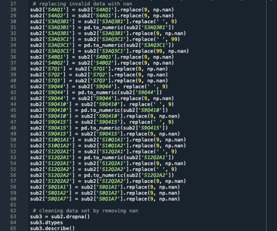
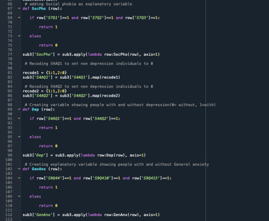
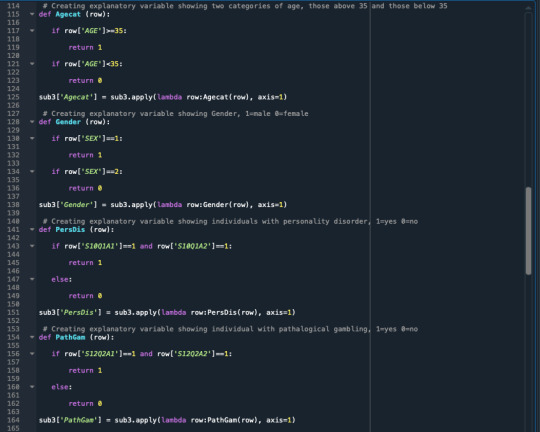
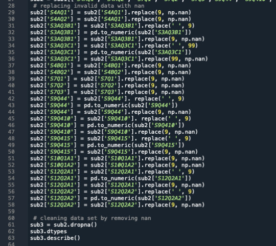
After cleaning the data by choosing the variables that we wanted for the study and removing any invalid data such as those that were unknows, descriptive information about the variables were generated. Figure 1 shows a descriptive statistic on the quantitative predictors that have been used in this study. It shows the counts, mean, standard deviation, minimum, 25th percentile, 50th percentile, 75th percentile, and maximum values for the predictors. The count shows that from the 59,400 water pumps, only 16,333 have been selected in this study after cleaning and filtering the data.

Figure 1: Descriptive statistics for quantitative predictors

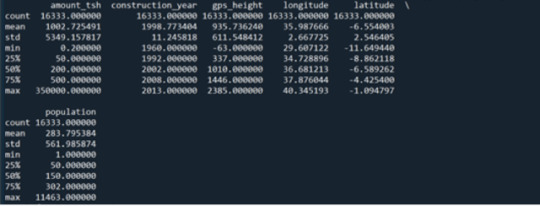
Figure 2 shows the frequency counts for the categorical explanatory variables.

Bivariate Analysis:

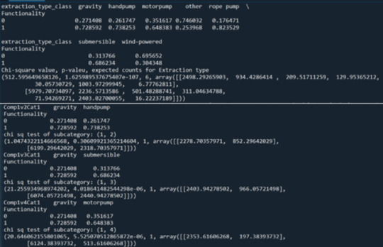
For the bivariate analysis, the chi-squared test of independence has been used after changing the quantitative variables to categorical. Column percentages and bar charts were then generated for each variable. Some variables consisted of more than two levels, therefore a post hoc test was needed in order to protect against type 1 error. The post hoc test used was the Bonferroni adjustment, which required the comparison between the levels of categorical variables one at a time. Figure 3 shows the column percentages, chi-square test of independence as well as the post hoc test on one of the explanatory categorical variables which was the “extraction_type_class”. The functionality of the pump has been coded so that 0=non-functional and 1=functional, so for the water pumps it can be seen that the most percentage of functioning pumps are the rope pump with 81.5% functionality. The chi-square value was quite high, which was 242.18, and the p-value was much lower than 0.05 therefore it shows that the result is significant. However, due to the variable consisting more than 2 levels, the Bonferroni Adjustment was made and the chi-square value has become less but still significant, and the adjusted p-value has increased but is still significant and shows a relationship between the predictor and the response variable even when other levels are controlled. Only some of the comparisons appeared to show an insignificant relationship such as that from chi-square test of subcategory (1, 5) which has a p-value of 0.0419 while the adjusted p-value should be less than 0.01 to be significant.

Figure 3: Column percentages, chi-square value, expected counts and post hoc test for extraction type

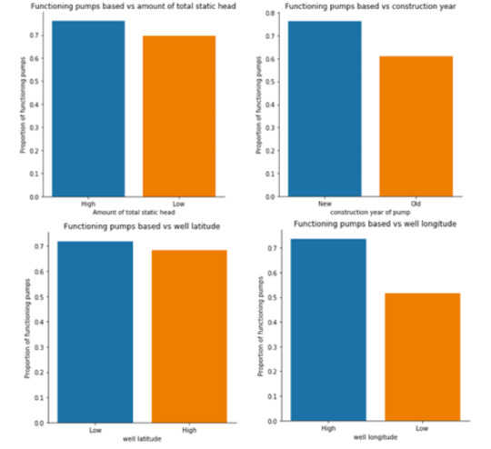
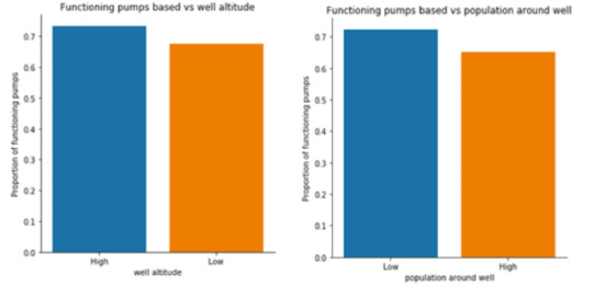
The chi-square test of independence has been generated for every predictor along with the post hoc test for explanatory variables with more than two levels. A total of twenty-eight comparisons were needed for the post hoc test of the extraction type. For the purpose of this report, the column percentages and chi-square test will not be shown for every individual variable, instead only the bar charts will be displayed for all the predictors. Figure 4 shows bar graphs of the functionality of the pumps against the original categorical predictors. Figure 5 shows bar graphs of the functionality of the pumps against the quantitative predictors that have been changed into categorical variables.

Figure 4: Original Explanatory predictors bar charts

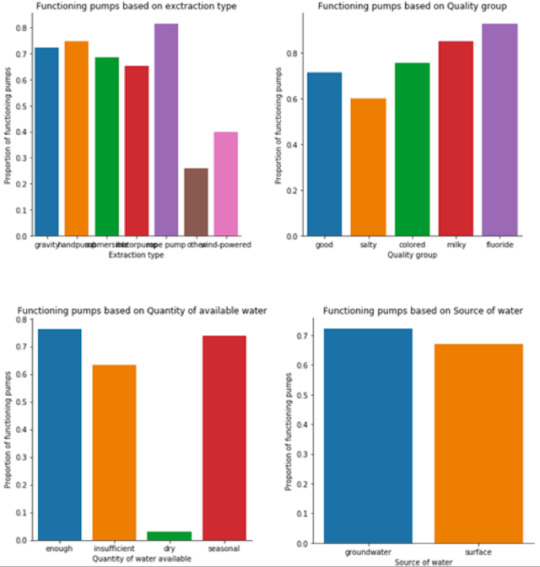
Figure 5: Original Quantitative predictors bar charts

Logistic Regression Model:

Figure 6 shows the logistic regression model that has been generated from the code. Most of the predictors seem to have a significant association with the response variable as their p-values are 0 or less than 0.05. Some of the variables such as the rose pump extraction type have been affected by lurking variables that increased their p-value from a significant value to 0.963. For the rose pump, the quantity of water was the lurking variable. We can also see that the predictors with the highest coefficient, which means has highest effect as the variable changes, is the quantity of water as they are 4.2099 and higher with a positive z value, while the rest of the predictors do not exceed 1.7. This shows that water pumps are 4.2099 more likely to be functional when placed in an area with insufficient water than when placed in a dry area. And it shows that water pumps are 4.7750 more likely to be functional when placed in an area with enough water than when placed in a dry area.

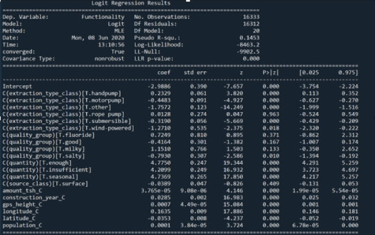
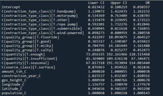
Figure 7 shows the odds ratios as well as the confidence intervals for the predictors. The predictors with the highest odds ratios can be seen to be the quantity of water available having an OR value of 118, 67, and 114. These values are significantly more than any other predictor. The quality group have some categories which have an OR value greater than 1 which is for the fluoride and the milky waters. However, from the p-value we can reject them as they are greater than 0.05.

Figure 7: Odds ratios and confidence intervals

MILESTONE 2

Sample

The sample that I have chosen includes N=14850 water pumps that were installed in Tanzania from the year 2011 to 2013. The data for this sample was collected by the Taarifa waterpoints dashboard, which aggregates data from the Tanzania Ministry of Water.

Measures

The usefulness of the water pumps was not chosen by the factors in the informational index yet were seen by the Tanzania Ministry of Water. There is an aggregate of 39 factors in the informational collection. Be that as it may, a few factors are like others and some are not identified with the investigation, hence they will be expelled from this examination. Rather, I will utilize just 10 of the 39 factors as indicators. The reaction variable a 3-level clear cut variable, however it has been binned into a 2-level all out factor which shows if the water siphon is useful or not.

The indicators incorporate 1) Total static head (measure of water accessible to waterpoint), 2) Construction year, 3) Altitude of well, 4) Longitude arrange, 5) Latitude facilitate, 6) Population around the well, 7) The sort of extraction the waterpoint utilizes, 8) The nature of the water, 9) Quantity of water, 10) Source class.

The vast majority of the indicators are quantitative factors, which are the all out static head, elevation of well, longitude arrange, and scope organize, and populace around the well. Concerning the remainder of the factors which are straight out factors, some have been decreased to a two-level unmitigated variable, for example, the nature of water and the amount of water. The source class is as of now a two-level straight out factor and the development year is a three-level downright factor. This lone leaves us with the extraction type which is a five-level clear cut variable, and this has been changed to be spoken to by sham codes.

Analysis

Since the indicators incorporate both quantitative and downright factors, a multiple regression model is utilized to decide the scientific connection between the indicators and the objective. The quantitative factors have been focused and the downright factors have been recoded to give it an estimation of zero. The coefficients and catches alongside the p-esteem are to be gathered and investigated. A q-q plot and a lingering plot will likewise be produced alongside an influence plot.

Subsequent to producing a numerous relapse model, an irregular forest will be created to all in all position the significance of the factors in foreseeing the objective of intrigue, which is if the water siphon is working or not. A preparation and test set will be utilized, in which the preparation set will comprise of 70% of the information, and the test set will comprise of 30% of the information.

MILESTONE ASSIGNMENT: 1

Title: An Algorithm for Predicting Functionality of Water Pumps in Tanzania.

Introduction to Research question:

The motivation behind this investigation is to distinguish the best indicators of the usefulness of water siphons in Tanzania, for example, scope, longitude, populace, water quality, and extraction strategy.

As a mechanical specialist, it is my obligation to offer types of assistance and keep up the usefulness of mechanical gadgets, for example, water siphons. Understanding the elements which influence the usefulness of these gadgets would permit me to anticipate when the gadget would glitch or need upkeep, and subsequently, we would have the option to give some support before this occurs. Playing out this errand would diminish the measure of time that siphons won't be working, and thus there would be more water accessible because of less shutdown time.

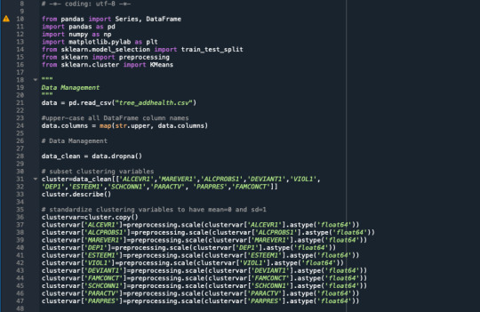
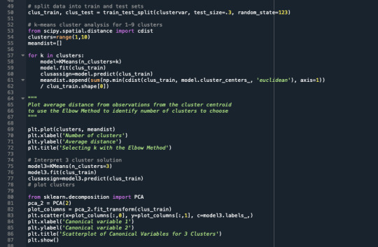
A k-means cluster analysis was conducted to identify underlying subgroups of adolescents based on their similarity of responses on 11 variables that represent characteristics that could have an impact on school achievement. Clustering variables included two binary variables measuring whether or not the adolescent had ever used alcohol or marijuana, as well as quantitative variables measuring alcohol problems, a scale measuring engaging in deviant behaviors (such as vandalism, other property damage, lying, stealing, running away, driving without permission, selling drugs, and skipping school), and scales measuring violence, depression, self-esteem, parental presence, parental activities, family connectedness, and school connectedness. All clustering variables were standardized to have a mean of 0 and a standard deviation of 1.

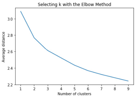
Elbow curve of r-square values for the nine cluster solutions

The elbow curve was inconclusive, suggesting that the 2, 4 and 8-cluster solutions might be interpreted. The results below are for an interpretation of the 4-cluster solution.

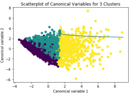
Canonical discriminant analyses was used to reduce the 11 clustering variable down a few variables that accounted for most of the variance in the clustering variables. A scatterplot of the first two canonical variables by cluster indicated that the observations in clusters 1 and 4 were densely packed with relatively low within cluster variance, and did not overlap very much with the other clusters. Cluster 2 was generally distinct, but the observations had greater spread suggesting higher within cluster variance. Observations in cluster 3 were spread out more than the other clusters, showing high within cluster variance. The results of this plot suggest that the best cluster solution may have fewer than 4 clusters, so it will be especially important to also evaluate the cluster solutions with fewer than 4 clusters.

Plot of the first two canonical variables for the clustering variables by cluster.

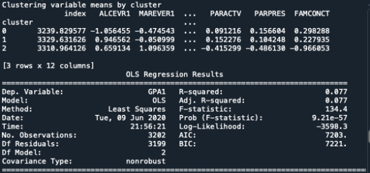
The means on the clustering variables showed that, compared to the other clusters, adolescents in cluster 1 had moderate levels on the clustering variables. They had a relatively low likelihood of using alcohol or marijuana, but moderate levels of depression and self-esteem. They also appeared to have fairly low levels of school connectedness parental presence, parental involvement in activities and family connectedness. With the exception of having a high likelihood of having used alcohol or marijuana, cluster 2 had higher levels on the clustering variables compared to cluster 1, but moderate compared to clusters 3 and 4. On the other hand, cluster 3 clearly included the most troubled adolescents. Adolescents in cluster three had the highest likelihood of having used alcohol, a very high likelihood of having used marijuana, more alcohol problems, and more engagement in deviant and violent behaviors compared to the other clusters. They also had higher levels of depression, lower self-esteem, and the lowest levels of school connectedness, parental presence, involvement of parents in activities, and family connectedness. Cluster 4 appeared to include the least troubled adolescents. Compared to adolescents in the other clusters, they were least likely to have used alcohol and marijuana, and had the lowest number of alcohol problems, and deviant and violent behavior. They also had the lowest levels of depression, and higher self-esteem, school connectedness, parental presence, parental involvement in activities and family connectedness.

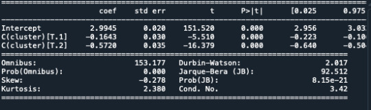
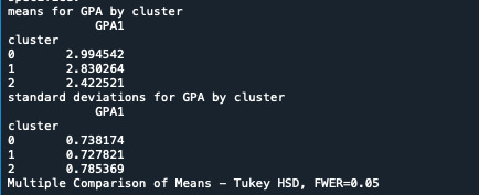
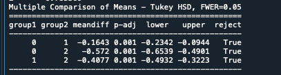
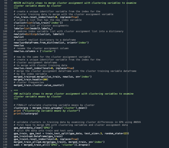
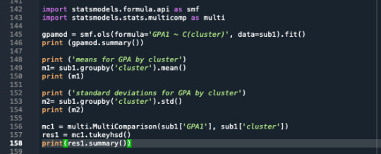
In order to externally validate the clusters, an Analysis of Variance (ANOVA) was conducting to test for significant differences between the clusters on grade point average (GPA). A tukey test was used for post hoc comparisons between the clusters. Results indicated significant differences between the clusters on GPA (F(3, 3197)=82.28, p<.0001). The tukey post hoc comparisons showed significant differences between clusters on GPA, with the exception that clusters 1 and 2 were not significantly different from each other. Adolescents in cluster 4 had the highest GPA (mean=2.99, sd=0.71), and cluster 3 had the lowest GPA (mean=2.36, sd=0.78).

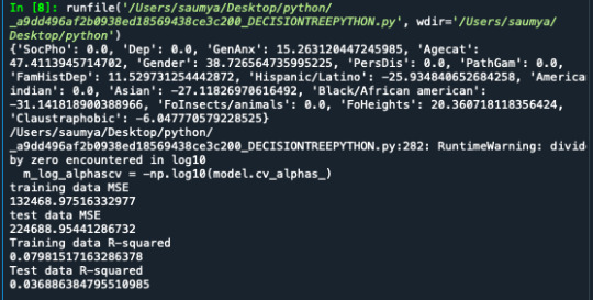
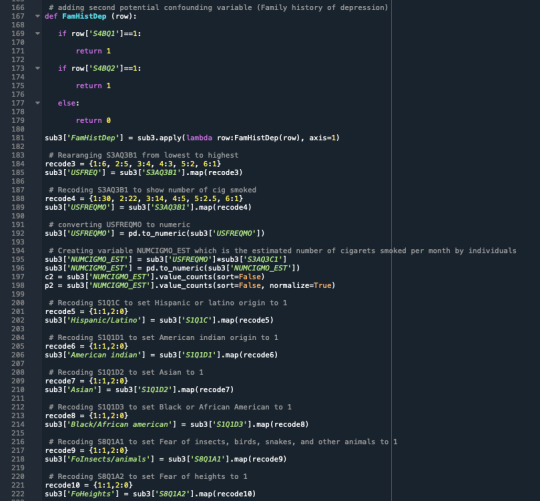
A tether relapse examination was directed to recognize a subset of factors from a sum of 15 unmitigated factors that best anticipate a quantitative reaction variable which is the evaluated number of cigarettes smoke by an individual for every month ("NUMCIGMO_EST). The indicators factors incorporate social fear, melancholy, general uneasiness, age(split into two classifications, those underneath and those over 35 years of age), character issue, obsessive betting, family ancestry of misery, Hispanic/Latino, American Indian, Asian, Black/African American, dread of bugs/creatures, dread of statures, and claustrophobic. A portion of the indicator factors are straight inquiries with parallel answers like "Asian", while others are controlled by a lot of answers like "Dep" which is despondency. All indicator factors were normalized to have a mean of zero and a standard deviation of one.

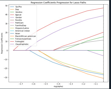
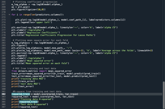
Information were haphazardly part into a preparation set that included 70% of the perceptions (N=526) and a test set that included 30% of the perceptions (N=226). In this code, I utilized the least point regression(LAR) calculation and included k=10 for the crease cross approval in which I showed to have 10 folds. In the yield area, the relapse coefficients are appeared for every one of the indicator factors, in which some have contracted to 0 like social fear and wretchedness. Age and sex had the most elevated positive coefficients and are related with number of cigarettes smoke, while dark/African American, Asian, and Hispanic/Latino had the most noteworthy negative coefficients and are adversely connected with the quantity of cigarettes smoked. This can likewise be appeared for the 'Relapse coefficients movement for Lasso Paths' plot.

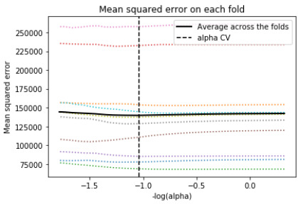
The last plot shows the mean squared mistake on each overlay. They are for the most part very high, and they don't change without question

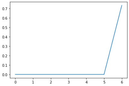
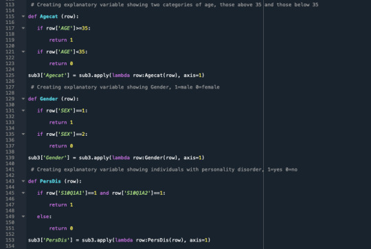
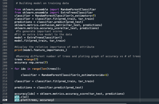
A random forest analysis was done to evaluate the importance of a series of explanatory variables in predicting a binary, categorical response variable. The explanatory variables were 6 categorical explanatory variables. The variables are social phobia, general anxiety, an age category split to 1= above 35 years and 0= less than 35 years old, gender 1=male, 0=female, personality disorder, and pathological gambling.

The graph produced shows us that we will get the most accurate results when we generate six trees, and the accuracy will be 0.698(approx.)

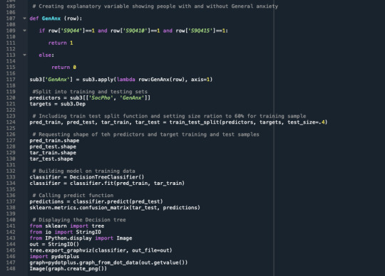
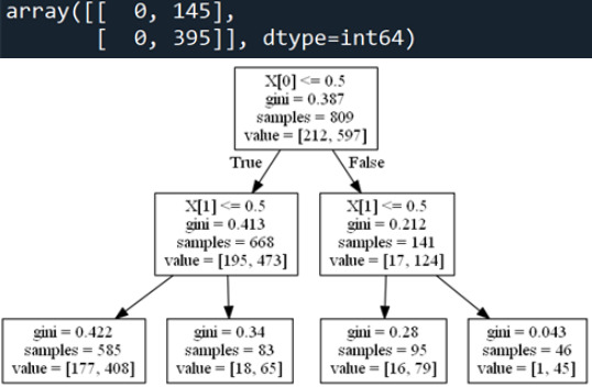
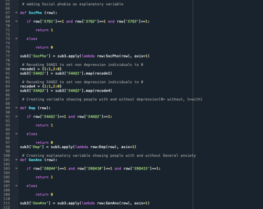
The choice tree investigation was performed to test the nonlinear connections among a progression of informative factors and a twofold clear cut reaction variable. The logical factors were Social fear and General tension, in which 0=no and 1=yes for both. The Response variable was Depression in which 0=no and 1=yes too. Social fear was the main variable to isolate the example into two subgroups. People without social fear , X[0]<=0.5, ended up being 668 out of 809 and went to one side of the principal subgroup. Individuals with social fear, X[0]>0.5, ended up being 141 out of 809 and were in the correct side of the primary subgroup. The second isolating variable was General nervousness, which split the example to a sum of four gatherings. The last subgroups shows that the all-out number of individuals who didn't experience the ill effects of social fear or general nervousness and don't have despondency are 177 out of 585, and those with discouragement are 408 out of 585. Concerning the far end to the correct indicating the individuals that experience the ill effects of social fear and general nervousness and don't have wretchedness are 1 out of 46, and those with discouragement are 45 out of 46. Taking the rates in the middle of, the individuals experiencing misery is expanding with each extra informative variable that is supposed to be yes. So from the last subgroup from the left side to the correct side, the level of individuals experiencing melancholy contrasted with its gathering is 69%, 78%, 83%, and 97% separately. This shows the logical factors do affect the reaction variable.

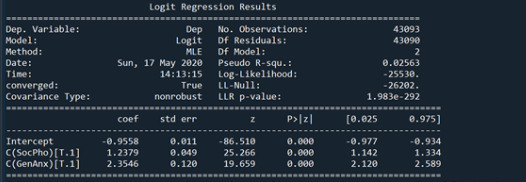
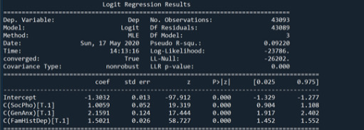
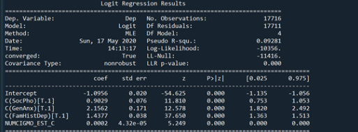
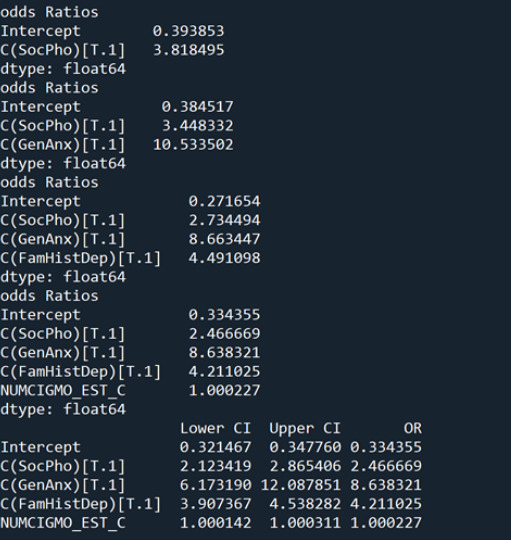
In this assignment, I am looking at the association between Social Phobia(my primary categorical explanatory variable) and Depression(my categorical response variable). While looking at these two variables I also add more explanatory variables to see if they are confounding or not, and these variables are “GenAnx”(general anxiety), “FamHistDep”(family history of depression), and “NUMCIGMO_EST_C”(number of cigarettes smoked per month after centering the data since it was a quantitative explanatory variable).

From the output shown above, I have included the logistic regression models for all of the explanatory variables after adding them one at a time to see their effects. As you can see in the fourth regression model, all of the explanatory variables seem to have an association with the response variable as they have a significant parameter estimate and a p value of 0.

odds ratio

I then generated the Odds Ratios after adding the explanatory variables one at a time to see their associations. It can be seen that every time I add an explanatory variable, the odds ratios decrease from the previous explanatory variable. For example, social phobia started with an OR of 3.81, but after adding all the explanatory variables it decreased to 2.46 which is still significant, but lower than what it started with. The final OR output shows that after accounting for all of the variables, all of the variables are associated with depression since their OR value is greater than 1, except for “NUMCIGMO_EST_C” which is almost 1 and therefore we can say that it is insignificant. As for the other variables, “SocPho” has an OR=2.46, “GenAnx” has an OR=8.63, and “FamHistDep” has an OR=4.21. Which shows that they are all significant values and they are associated with depression. So people with social phobia are 2.46 times more likely to have depression than people without social phobia. People with general anxiety are 8.63 more times likely to have depression. And people with a family history of depression are 4.21 times more likely to have depression.

At the end of the code, I generated a confidence interval which shows were estimate 95% of the population parameter to fall in. As can be seen, all explanatory variables have valid confidence intervals expect for “NUMCIGMO_EST_C”.

Therefore, we can social phobia, general anxiety, and a family history of depression are all associated with depression. Therefore, we can reject the null hypothesis in that there is no association between the explanatory and response variable in this case. The number of cigarettes smoked per month is not associated with depression. Thus we can accept the null hypothesis for this variable.

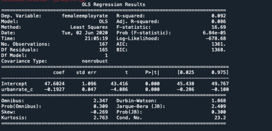
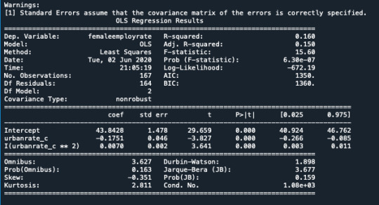
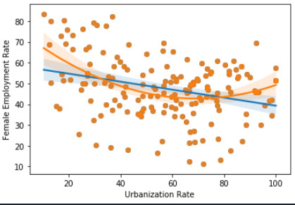
1.Negative linear coefficient and positive quadratic coefficient so Curve is convex

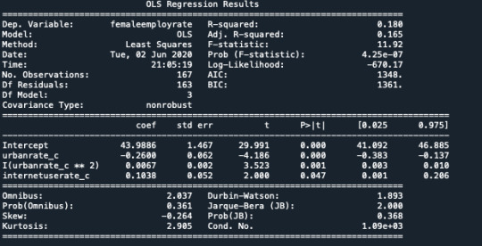
2.After adding internet use rate all the coefficients are significant.

q-q plot (for seeing residual are normally distributed)

residuals follow straight line but deviate at the start and end of the line

which means that there is not a proper normal distribution among the residual

therefore, other residuals can be added to see the true distribution and helps In understanding the model.

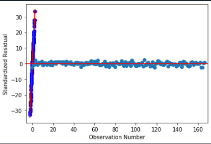
standardize residual plot

the distribution of residual fall in a normal distribution to the mean. Most of them lies in a straight line at 0 and at observing number 0 there is a straight vertical line.

All lie between -1 to 1 and others can consider as outliners. Model can be accepted but could be improved.

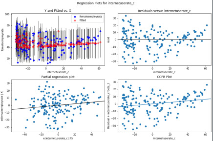
Regression plots - Module do not predict female employment rate right when we compare it with internet use rate because of the shapes of graphs.

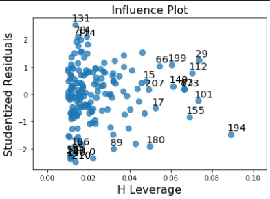
Leverage plot

Leverage lies between -2 to 2 and points greater than 2 or -2 are less and even lie on the left side of the plot that means it does not have undue influence on the estimates of th regression model

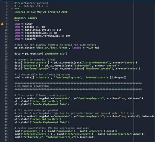
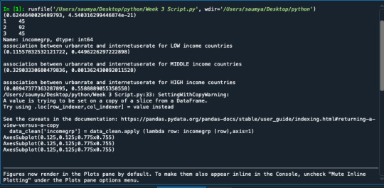
The coefficient for urbanrate is 0.72, and the intercept is -4.90. So now we know that our equation for the best fit line of this graph is Internet user rate equals - 4.90 +0 .72 times urban rate.The p value is 0.000 which means that it's really small. Here you would report the p value p<.0001.

DATA ANALYSIS

SAMPLE

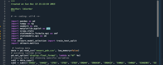
The example is from the primary influx of the National Epidemiologic Survey on Alcohol and Related Conditions (NESARC), the biggest across the country longitudinal review of liquor and medication use and related mental and clinical comorbidities. Members (N=43,093) spoke to the regular citizen, non-standardized grown-up populace of the United States, and

included people living in families, military staff living misguided, and people living in the accompanying gathering quarters: boarding or staying houses, non-transient lodgings and inns, covers, offices for lodging laborers, school quarters, and gathering homes. The NESARC included over testing of Blacks, Hispanics and youthful grown-ups matured 18 to 24 years. The information scientific example for this investigation included members 18-25 years of age who detailed smoking at any rate 1 cigarette for each day in the previous 30 days (N=1,320).

PROCEDURE

Information were gathered via prepared U.S. Registration Bureau Field Representatives during 2001–2002 through PC helped individual meetings (CAPI). One grown-up was chosen for meet in every family unit, and meetings were led in respondents' homes following educated assent techniques.

MEASURES

Lifetime significant wretchedness (for example those accomplished in the previous a year and before the previous a year) was surveyed utilizing the NIAAA, Alcohol Use Disorder and Associated Disabilities Interview Schedule – DSM-IV (AUDADIS-IV) (Grant et al., 2003; Grant, Harford, Dawson, and Chou, 1995).

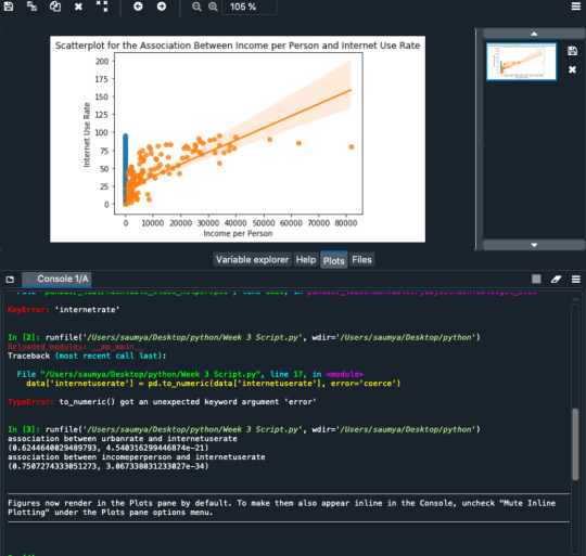
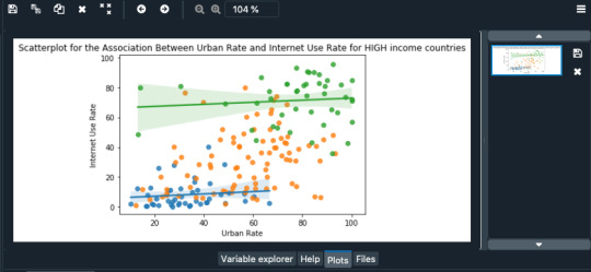
the relationship between urban rate and internet use rate, r= 0.61, we get r^2 0.37. This could be interpreted the following way. If we know the urban rate, we can predict 37% of the variability we will see in the rate of internet use. Of course, that also means that 63% of the variability is unaccounted for. If we see r^2 for income per person and internet use rate, we get a value of 0.56. This suggests if we know income per person, we can predict 56% of the variability we'll see in the rate of internet use.

Model Interpretation for CHI-SQUARE TEST

When the association between the income level of an adults(categorical variable) and depression (categorical variable), a chi-square test of independence revealed that among the different level of income  people with low most likely to have high depression as compared to  those who have high level of income.

Thus the null hypothesis i.e the depression is not related to income is rejected.

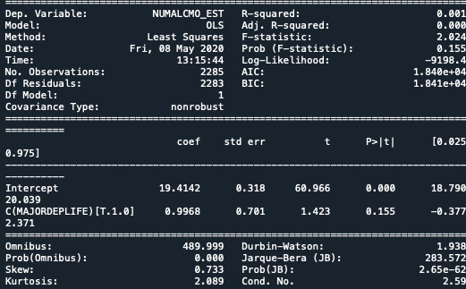
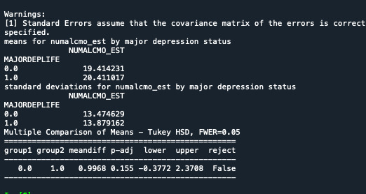
Model Interpretation for ANOVA tests

When the association between the number of alcohol drank by the young teenage adults(quantitative variable) and depression (categorical variable), we can make out that those with depressed people has drank nearly more(MEAN =±20.41,STD=±13.87) than the ones without depression(MEAN=±19.41,STD=±13.47).

In my experiment, the actual F value is 2.024 and the probability p < 0.155.

Model Interpretation for post hoc ANOVA results

ANOVA revealed that the number of number r of drinks (quantitative variable) and the depression (categorized variable) were associated to each other(F=2.024 and p=0.155), so we can accept the null hypothesis.

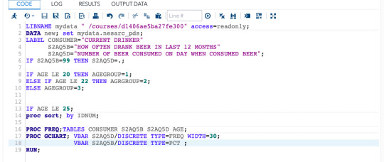
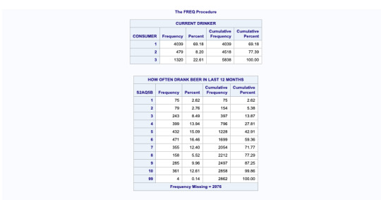
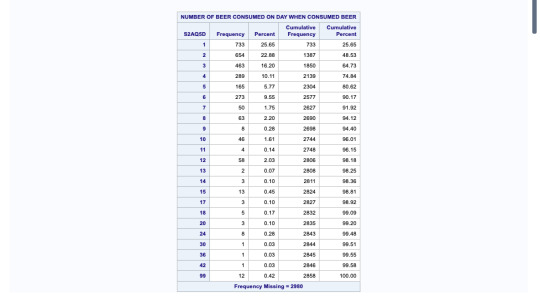
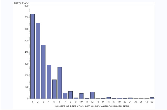
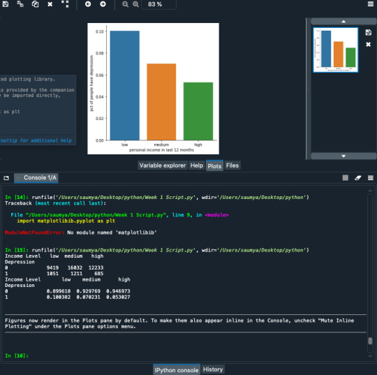
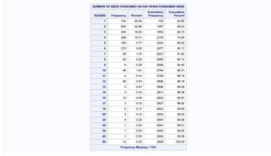
this SAS data shows us the codes and data which is represented in graphical manner. The graphs are shown of “how often drank beer in last 12 months” in percentage and “number of beer consumed on day when consumed” in frequency.

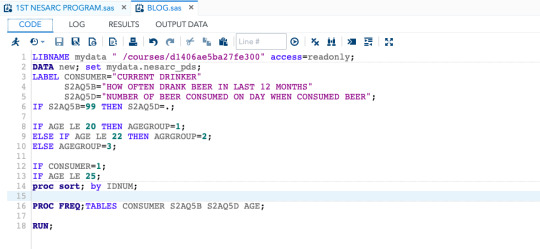
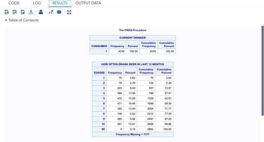
This SAS language shows us the data of beer consumers it includes missing data we did not get at the time of interview as it was a skipped question, codes of all the in valid data is shown, grouping/binning of variable is also shown by grouping ages into different category.