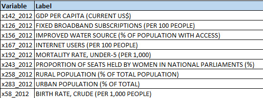
The Association between GDP Per Capita and Various Development Indicators

Introduction to the Research Question The purpose of this study was to identify the best predictors of a country’s GDP per capita from multiple indicators common to development goals, that is, fixed broadband subscription rate, access to improved water sources, internet user rate, mortality rate for under 5-year old, proportion of seats held by women in national parliaments, rural population rate, urban population rate, and the birth rate. I spent spent my career living in developing countries while working for an international aid agency. By investigating which development goals most effectively lead to increases in GDP per capita, all aid agencies globally will be better able to focus their activities towards improvement of those indicators, which will indirectly lead to increased incomes for families. I have witnessed firsthand how a small income boost to impoverished communities can lead dramatic improvement in quality of life in those communities. By focusing development efforts on improving the indicators which are most closely correlated to GDP per capita, aid agencies can have the greatest impact towards their end goals.

Methods

Sample The World Bank data set is a subset of data extracted from the primary World Bank collection of development indicators, compiled from officially-recognized international sources, from the years 2012 and 2013. The sample used in this study contained N = 248 countries with data aggregated from national, regional, and global estimates. Although all variables have valid data observations for a minimum of 190 countries, only data from the year 2012 was used in this study because this was not intended to be a longitudinal study. Furthermore, 2013 data has been reserved to test the regression equation developed by the 2012 data for validity. Measures The GDP per capita, in current US dollars, is the quantitative response variable. Gross Domestic Product is a measure of output of a country, created by taking the monetary value of all finished goods and services produced within the country’s borders during a specific time period, and dividing it by the country’s population. It is a commonly used indicator of standard of living, with higher GDP per capita equating to a higher standard of living.

Predictors used in the study are all quantitative, and they are:

Analyses Because all variables are quantitative, the distributions for the predictors and the GDP per capita response variable were evaluated by calculating the mean, standard deviation, and minimum and maximum. A scatter plot for each variable was also examined, and a Pearson correlation was used to test bivariate associations between the individual quantitative predictors and the GDP per capita response variable. Many plots appeared to display a logarithmic relationship between the predictor and response, so a Pearson correlation was calculated from the log of the predictor and the response. When the log correlation was more significant than the linear correlation, the log relationship was reported. 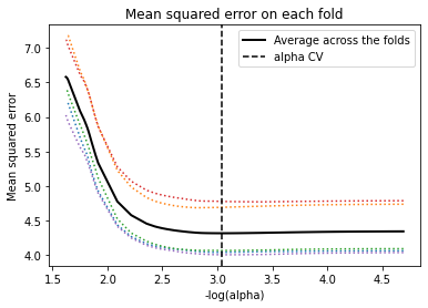Lastly, a lasso regression with the least angle regression selection algorithm was used to identify the subset of variables that best predicted GDP per capita. The lasso regression model was estimated on a training data set consisting of the 2012 data (N = 248) and tested on the 2013 data. All predictor variables were standardized to have a mean = 0 and standard deviation = 1 prior to conducting the lasso regression analysis. Cross validation was performed using k-fold cross validation specifying 10 folds. The change in the cross validation mean squared error rate at each step was used to identify the best subset of predictor variables. Predictive accuracy was assessed by determining the mean squared error rate of the training data prediction algorithm when applied to observations in the test data set.

RESULTS:

Descriptive Statistics Table 1 shows descriptive statistics for GDP per capita and the quantitative predictors. The average GDP per capita was US$ 14,751 (std dev = 21,612) with a minimum GDP of US$ 244.2 and a maximum of US$ 149,161

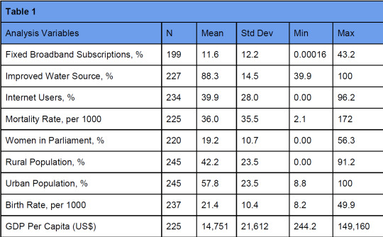
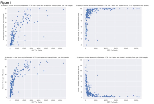
Bivariate Analyses Scatter plots for the association between the GDP per capita response variable and the quantitative predictors (Figure 1) revealed that GDP per capita has the strongest correlation with the rate of fixed broadband subscriptions (Pearson r = 0.789, p < .0001). All correlations are shown in Table 2.

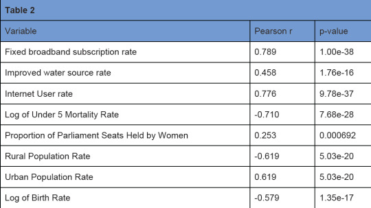
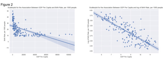
Note that the Under 5 Mortality Rate was transformed to a logarithmic scale in order to linearize it for more accurate regression analysis. Figure 2 shows the scatterplot resulting from this transformation, showing the increased linearity.

Lasso Regression Analysis: Of the 8 predictor variables analyzed, the lasso regression model dropped 2 of them. The proportion of women in national parliament was not retained (the regression analysis also showed it to have the least significance by a wide margin), and the rural population rate was not retained (the urban population rate captures the same information, in the inverse, and also had a slightly higher correlation than the rural population rate; the urban population rate was retained). Table 3 shows the regression coefficients of the lasso analysis.

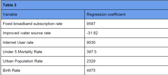
GDP per capita increases the most with the fixed broadband subscription rate and the linked variable of internet user rate. The weakest predictor retained in the model was the rate of access to an improved water source. Indeed, nearly all of the countries in the survey have a 100% rate, so not much information was provided by this data point. Together, these 6 variables can explain 68% of the variability of GDP per capita (Training data R-square = 0.6827; Test data R-square = 0.6806). The mean squared error for the training set was 124390237 and for the testing set was 123487565.

GDP per capita increases the most with the fixed broadband subscription rate and the linked variable of internet user rate. The weakest predictor retained in the model was the rate of access to an improved water source. Indeed, nearly all of the countries in the survey have a 100% rate, so not much information was provided by this data point. Together, these 6 variables can explain 68% of the variability of GDP per capita (Training data R-square = 0.6827; Test data R-square = 0.6806). The mean squared error for the training set was 124390237 and for the testing set was 123487565.

Conclusion and Limitations:

This project used lasso regression analysis to identify a subset of development-related variables that best predicted Gross Domestic Product per capita in N = 248 countries and regions in the world during the year 2012. GDPs per capita ranged from $244 to $150,000, indicating that there was considerable variability in the distribution of incomes around the world. The lasso regression analysis indicated that 6 of the 8 development-related predictor variables were selected in the final model. These 6 predictors accounted for 68% of the observed variability in GDPs per capita. Only the rural population rate and proportion of seats held by women in national parliaments were excluded. The strongest predictors of GDPs per capita were the fixed broadband subscription rate and the internet user rate. GDPs per capita were greater when both fixed broadband subscription rates and internet user rates increased. Access rates to improved water sources paradoxically emerged as a predictor of lower GDPs per capita, but the regression coefficient is small relative to the other predictors, so the effect is negligible. There was a slight decrease in the mean squared error when the 2012 set lasso regression algorithm was used to predict GDPs per capita in the 2013 set. This suggests that the predictive accuracy of the algorithm may be stable in future samples of GDPs per capita.

The results of this project indicate that efforts to increase internet penetration rates and get more users connected in a country are a priority for achieving consistently higher GDPs per capita. These results should be considered carefully when deciding how to spend development aid money. Although higher GDPs per capita are frequently used as a proxy measure for higher quality-of-life, other indicators such as mortality rates and access to trade markets for goods and services indirectly lead to higher GDPs per capita but directly lead to higher quality-of-life. Therefore, if aid money is to be spent on increasing internet penetration rates, it must be done so minimally so that aid funds remain available to be spent on other indicators. Although access rates to improved water sources and birth rate were both retained in the final lasso regression model, Table 2 showed that the bivariate analyses indicated these variables to be only weakly correlated with GDP per capita. Table 3 shows that the lasso regression model did not weigh these predictors highly in the final model. This suggests that these two development-related factors may not have a considerable impact on GDPs per capita, and re-analysis of these factors should be conducted on future datasets to determine whether this conclusion is supported. This project successfully developed a predictive algorithm for GDPs per capita that appears to have little bias and variance in a different sample. In addition, it provides more information on which development-related factors are most likely to have a significant impact on GDPs per capita. However, there are some limitations that should be taken into account when considering changes in the way funds are spent in the international development field based on the results of this project.

First, we analyzed only data from a single year, but development of countries is ongoing. So, it is important to test this algorithm on datasets that are surveyed in multiple years to determine whether the algorithm remains relatively unbiased and stable despite these ongoing changes.

Second, the analysis was conducted on only a subset of the available development data. Different factors may emerge as the important predictors of GDPs per capita when using the full collection of potential predictors. Therefore, we cannot assume that the predictive algorithm developed in this study will be the best possible when different development indicators available.

Finally, there is a large number of development-related factors that could impact GDPs per capita, but the current project examined only a few of these factors. It is possible that the factors identified as important predictors of GDPs per capita among the set of predictors analyzed in this project are confounded by other factors not considered in this analysis. As a result, these same factors may not emerge as important factors when other factors are taken into consideration. Therefore, future efforts to develop a solid predictive algorithm for GDPs per capita should expand the algorithm by adding more development-related predictors to the statistical model, and evaluating the applicability of the algorithm with this greater dataset.

Running a k-means Cluster Analysis

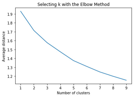
A k-means cluster analysis was conducted to identify subgroups of traffic collisions in my city based on their similarity of time attributes that could have an impact on the severity. Clustering variables included quasi quantitative variables representing year, month, day and hour. All clustering variables were standardized to have a mean of 0 and a standard deviation of 1.

Data were randomly split into a training set that included 70% of the observations (N=3091) and a test set that included 30% of the observations (N=1325). A series of k-means cluster analyses were conducted on the training data specifying k=1-9 clusters, using Euclidean distance. The variance in the clustering variables that was accounted for by the clusters (r-square) was plotted for each of the nine cluster solutions in an elbow curve to provide guidance for choosing the number of clusters to interpret.

Canonical discriminant analyses was used to reduce the 4 clustering variables down to two variables that accounted for most of the variance in the clustering variables.

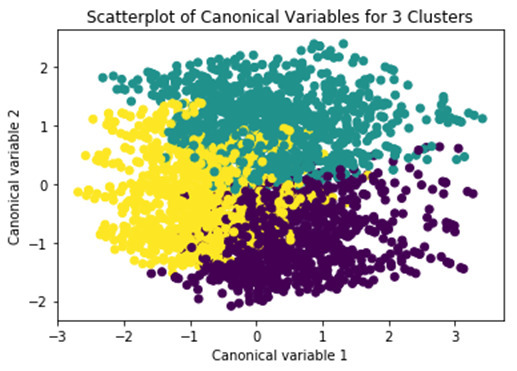
Clustering variable means by cluster

              index      Year     Month       Day      Hour

cluster                                                    

0       2245.346918  0.701135 -0.003901 -0.826094 -0.143868

1        2134.100881  0.473399 -0.073513  0.925436 0.326646

2        2244.270677 -1.159774  0.057375 -0.052790 -0.158900

 Cluster 1 shows higher likelihood of a later day in the week attribute and at a later time of day attribute..

Lasso Regression

A lasso regression analysis was conducted to identify a subset of variables from a pool of 23 categorical and quantitative predictor variables that best predicted a quantitative response variable measuring family connectedness in adolescents. Categorical predictors included gender and a series of 5 binary categorical variables for race and ethnicity (Hispanic, White, Black, Native American and Asian) to improve interpretability of the selected model with fewer predictors. Binary substance use variables were measured with individual questions about whether the adolescent had ever used alcohol, marijuana, cocaine or inhalants. Additional categorical variables included the availability of cigarettes in the home, whether or not either parent was on public assistance and any experience with being expelled from school. Quantitative predictor variables include age, alcohol problems, and a measure of deviance that included such behaviors as vandalism, other property damage, lying, stealing, running away, driving without permission, selling drugs, and skipping school. Another scale for violence, one for depression, and others measuring self-esteem, parental presence, parental activities, school connectedness and grade point average were also included. All predictor variables were standardized to have a mean of zero and a standard deviation of one.

Data were randomly split into a training set that included 60% of the observations (N=3201) and a test set that included 40% of the observations (N=1701). The least angle regression algorithm with k=5 fold cross validation was used to estimate the lasso regression model in the training set, and the model was validated using the test set. The change in the cross validation average (mean) squared error at each step was used to identify the best subset of predictor variables.

Of the 23 predictor variables, 12 were retained in the selected model. During the estimation process, self-esteem and parental activities were most strongly associated with family connectedness, followed by parental presence and engaging in violent behavior. Age, Cigerrate availability, Depression, use of inhalants and marijuana were negatively associated with family connectedness and self-esteem, gender were positively associated with family connectedness.

Running a random forest

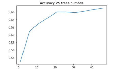
Random forest and ExtraTrees classifier were deployed to evaluate the importance of a series of explanatory variables in predicting a categorical response variable - red wine quality (score between 0 and 10). The following explanatory variables were included: fixed acidity, volatile acidity, citric acid, residual sugar, chlorides, free sulfur dioxide, total sulfur dioxide, density, pH, sulphates and alcohol.

The explanatory variables with the highest importance score (evaluated by both classifiers) are alcohol, volatile acidity, sulphates. The accuracy of the Random forest and ExtraTrees clasifier is about 67%, which is quite good for highly unbalanced and hardly distinguished from each other classes. The subsequent growing of multiple trees rather than a single tree, adding a lot to the overall score of the model. For Random forest the number of estimators is 20, while for ExtraTrees classifier - 12, because the second classifier grows up much faster.

Running a Classification Tree

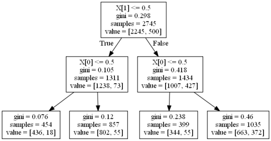
Decision Tree analysis was performed to test non-linear relationships among a set of explanatory variables and a binary categorical response variable.

The following explanatory variables were included as possible contributors to a classification tree model evaluating regular smoking (the response variable): Color (White/Black) and use of alcohol.

The color  was the first variable to separate the sample into two subgroups. White people were more likely to be non-regular smokers than black people, although by a narrow margin.

Further subdivisions were made based on alcohol use. Among 454 white people who regularly used alcohol, 436 white people who were non-regular smokers while 18 were regular smokers. Among the 857 of whites who were non users of alcohol, 802 were non-regular smokers while 55 were regular smokers. Among 1035 black people who used alcohol, 344 were non-regular smokers while 55 were regular smokers, and among the 1035 black people who were non users of alcohol, 663 black people were non regular smokers while 372 were regular smokers.

Writing About Your Data

The data was provided by the National Epidemiological Survey on Alcohol and Related Conditions (NESARC), which was conducted in a random sample of 43,093 U.S. adults and designed to determine the magnitude of alcohol use and psychiatric disorders. Sample size is important because the larger the sample size, the more accurate the findings. NESARC’s unusually large sample size also made it possible to achieve stable estimates of even rare conditions. NESARC participants came from all walks of life and a variety of ages, and the level of analysis studied was individual. They represented all regions of the United States and included residents of the District of Columbia, Alaska, and Hawaii. In addition to sampling individuals living in traditional households, NESARC investigators questioned military personnel living off base and people living in a variety of group accommodations such as boarding or rooming houses and college quarters. More specifically, the sample consists of 24,575 (57.1%) males and 18,518 (42.9%) females, among of whom 9,535 (22.13%) were aged between 18 and 30 years old. The data analytic subset, examined in this study, includes individuals aged between 18 and 30 years old who reported using cannabis at least once in their life (N=2,412).

Procedure

In 2001—2002, the National Institute on Alcohol Abuse and Alcoholism (NIAAA) conducted the first wave of the National Epidemiological Survey on Alcohol and Related Conditions (NESARC), the largest and most ambitious survey of this type conducted to date. Information was collected in face-to-face computer-assisted interviews, which took place in the participants’ homes. It contained an extensive battery of questions about present and past alcohol consumption, AUDs, and the use of alcohol treatment services. NESARC also included similar questions related to tobacco and illicit drug use (including nicotine dependence and drug use disorders), as well as questions designed to determine a wide variety of psychiatric disorders such as major depression, anxiety disorders, and personality disorders. The original purpose of this survey was to evaluate the magnitude and have a better understanding of the link between alcohol use and other drug use and/or psychiatric disorders, which can help treatment providers design more targeted screening and more effective treatments for their patients. The response rate was 81%, which is significantly high compared to the standards of recent large-scale national surveys. A high response rate is very important, since it is key to legitimizing the results of the survey.

Logistic Regression Model

Preview

This assignment aims to examine the association of potential drug abuse/dependence prior to the last 12 months with major depression diagnosis in the last 12 months. among US adults aged from 18 to 30 years old (N=9535). All four explanatory variables were 4-level categorical and they were binned into 2 categories (0.=“No abuse/dependence, 1.=“Drug abuse/dependence”) for the purpose of these logistic models. More specifically, cannabis abuse/dependence (CANDEPPR12) is the primary explanatory variable and the potential confounding factors were cocaine (COCDEPPR12), heroine (HERDEPPR12) and alcohol (ALCDEPPR12). The response variable is major depression (MAJORDEP12) diagnosed in the last 12 months, which is categorical binary variable (0.=“No”, 1.=“Yes”). Therefore, we can evaluate if a specific drug abuse/dependence issue during the period prior to the last 12 months, is positively correlated with depression diagnosis in the last 12 months.

RESULTS

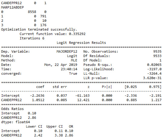
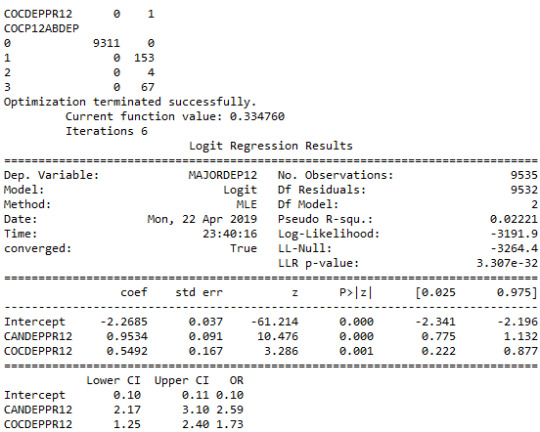
The logistic regression model presented above illustrates the association of cannabis and cocaine abuse/dependence issue prior to the last 12 months with major depression, diagnosed in the last 12 months. The number of observations is 9535 (18-30) and the regression is significant at a P value of less than 0.0001 for cannabis and 0.001 for cocaine. The odds of having major depression were 2.5 times higher for participants with cannabis abuse/dependence than for participants without abuse/dependence (OR=2.59, 95% CI = 2.17-3.10, p=.0001). For cocaine the odds of having major depression were more than 1.7 times higher for individuals with cocaine abuse/dependence than for individuals without abuse/dependence (OR=1.73, 95% CI = 1.25-2.40, p=.001).

On the other hand, heroine’s relationship with major depression was not significant, with a p-value at 0.079 which is more than 0.05. Thus, the null hypothesis cannot be rejected.

After adjusting for potential confounding factors alcohol and cocaine abuse/dependence, the odds of having depression were slightly more double for participants with cannabis issues than for participants without cannabis issues (OR=2.11, 95% CI = 1.74-2.55, p=.0001). Alcohol appeared to be also positively correlated with major depression, since alcoholic individuals had 1.5 times higher odds of getting diagnosed with this psychiatric disorder (OR=1.5, 95% CI = 1.32-1.79, p=.0001). Cocaine’s abuse/dependence odds seemed to be very close to alcohol (OR=1.54, 95% CI = 1.11-2.14, p=.01).

SUMMARY

The logistic regression model revealed that cannabis, cocaine and alcohol were positively correlated with major depression, while heroine was not. Cannabis dependence was my primary explanatory variable and its significance appeared to remain steady when adding potential predictors (alcohol and cocaine) to the model. Therefore, there was no evidence of confounding for the association between my primary explanatory variable and the response variable. The results support my initial hypothesis.

Multiple Regression Model

The multiple regression analysis aims to evaluate multiple predictors of the quantitative response variable, number of cannabis dependence symptoms (CanDepSymptoms). The primary explanatory variable is major depression diagnosis, in the last 12 months (MAJORDEP12), while the confounding factors are:

agebeganuse_c: Centered quantitative variable, which represents the age when individuals began using cannabis the most (values 5-64. Age).

numberjosmoked_c: Centered quantitative variable, which represents the number of joints smoked per day when using cannabis the most (values 1-98. Joints).

canuseduration_c: Centered quantitative variable, which represents the duration (in weeks) individuals used cannabis the most (values 1-2818. Weeks).

GENAXDX12: Categorical variable, which represents the diagnosis of general anxiety in the last 12 months (0.=“No”, 1.=“Yes”).

DYSDX12: Categorical variable, which represents the diagnosis of dysthymia in the last 12 months (0.=“No”, 1.=“Yes”).

SOCPDX12: Categorical variable, which represents the diagnosis of social phobia in the last 12 months (0.=“No”, 1.=“Yes”).

After adjusting the potential confounding factors, major depression (Beta=0.25, p=0.0001) was significantly and positively associated with number of cannabis dependence symptoms. The R-squared value was extremely small at 0.047 and F-statistic value is equal to 16.88. For the confounding variables:

Age when began using cannabis the most was not significantly associated with cannabis dependence symptoms and the null hypothesis cannot be rejected (Beta=-0.03, p=0.18).

Number of joints smoked per day was significantly associated with cannabis dependence symptoms, such that the larger quantity reported a greater number of cannabis dependence symptoms (Beta= 0.003, p=0.008).

Duration of cannabis use was not significantly associated with cannabis dependence symptoms and the null hypothesis cannot be rejected (Beta=9.4e-06, p=0.56).

General anxiety diagnosis was not significantly associated with cannabis dependence symptoms and the null hypothesis cannot be rejected (Beta=0.18, p=0.07).

Dysthymia diagnosis was significantly associated with cannabis dependence symptoms (Beta= 0.43, p=0.0001).

Social phobia diagnosis was significantly associated with cannabis dependence symptoms (Beta= 0.31, p=0.0001).

Report

To evaluate if the additional explanatory variables confounded the relationship between major depression diagnosis (primary explanatory variable) and cannabis dependence symptoms (response variable), I added the variables to my model one at a time. As a result, none of this variables confounded the association, since every time I added each predictor the p-value of major depression remained significant, at 0.0001. Therefore, the results of the multiple regression analysis for these adjusted potential confounding variables, supported my initial hypothesis.

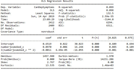
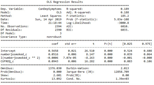
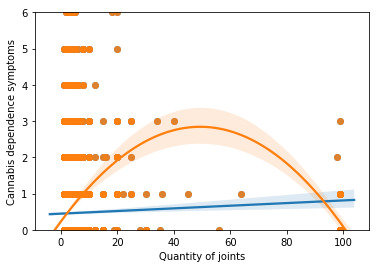
The second multiple regression analysis examines the association between the quantitative response variable, number of cannabis dependence symptoms (CanDepSymptoms) and the centered quantitative explanatory variable, number of joints smoked per day when using the most (numberjosmoked_c). A second order polynomial of number of joints variable (’numberjosmoked_c^2) was added to the regression equation in order to improve the fit of the model and capture the curve of linear relationship that was evident in the scatter plot. In addition, the recoded variable (CUFREQ) which represents the frequency of cannabis use (values 1-10, 1.=“Once a year”, 10.=“Every day”), was included to the model as a potential confounding factor. There is also a show that coefficients for the linear, and quadratic variables, remain significant after adjusting for frequency of cannabis use rate.

If we look at the results, it is noticeable that the value for the linear term for number of joints is 0.05, and the p value is less than 0.0001. In addition, the quadratic term is negative (-0.0006) and the p value is also significant (0.0001). The R square increases from 0.003 to 0.18., which means that adding the quadratic term for cannabis joints, increase the amount of variability in cannabis dependence symptoms that can be explained by cannabis use quantity from 0.3% to 18%. For the frequency of cannabis use the coefficient is equal to 0.09 and the p-value is significantly small, at 0.0001.

Diagnostic Plots

Q to Q Plot

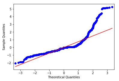
This qq-plot evaluates the assumption that the residuals from our regression model are normally distributed. A qq-plot, plots the quantiles of the residuals that we would theoretically see if the residuals followed a normal distribution, against the quantiles for the residuals estimated from the regression model. It is noticeable that the residuals generally deviate from a straight line, especially at higher quantiles. This indicates that our residuals did not follow perfect normal distribution. This could mean that the curvilinear association that we observed in our scatter plot may not be fully estimated by the quadratic cannabis joints variable. Therefore, there might be other explanatory variables that could improve estimation of the observed curvilinearity.

Plot of standardized residuals for all observations

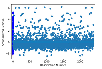
To evaluate the overall fit of the predicted values of the response variable to the observed values and to look for outliers, I created a plot for the standardized residuals of each observation. As we can see, most of the residuals fall between -2 and 2, but many of them fall also above 2. This indicates that we have several outliers, basically above the mean of 0. Furthermore, some of these outliers fall above 4 (extreme outliers) which suggests that the fit of the model is relatively poor and could be improved.

Regression plots for frequency of cannabis use

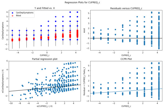
The plot in the upper right hand corner shows the residuals for each observation at different values of cannabis use frequency rate. There is clearly a funnel shaped pattern to the residuals where we can see that the absolute values of the them are small at lower values of frequency use rate, but then they start to get larger at higher levels. This indicates that this model does not predict cannabis dependence symptoms as well for individuals who have either high or low levels of cannabis use frequency rate. But is particularly worse predicting dependence symptoms for individuals with high frequency of cannabis use.

The partial regression residual plot, in the lower left hand corner, attempts to show the effect of adding cannabis use frequency rate as an additional explanatory variable to the model. For the frequency use rate variable, the values in the scatter plot are two sets of residuals. The residuals from a model predicting the cannabis dependence symptoms response from the other explanatory variables, excluding frequency of use, are plotted on the vertical access, and the residuals from the model predicting frequency of use from all the other explanatory variables are plotted on the horizontal access.What this means is that the partial regression plot shows the relationship between the response variable and specific explanatory variable, after controlling for the other explanatory variables. The residuals are spread out in a random pattern around the partial regression line and many of the residuals are pretty far from this line, indicating a great deal of cannabis dependence symptoms prediction error. Although cannabis use frequency rate shows a statistically significant association with cannabis dependence symptoms, this association is pretty weak after controlling for the number of joints smoked.

Leverage plot

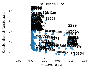
The leverage plot attempts to identify observations that have an unusually large influence on the estimation of the predicted value of the response variable, cannabis dependence symptoms, or that are outliers, or both. We can see in the leverage plot is that we have a several outliers, contents that have residuals greater than 2 or less than -2. We’ve already identified some of these outliers in previous plots, but the plot also tells us which outliers have small or close to zero leverage values, meaning that although they are outlying observations, they do not have an undue influence on the estimation of the regression model.

Basic Linear Regression Model

Preview

The data was provided by the National Epidemiological Survey on Alcohol and Related Conditions (NESARC), which was conducted in a random sample of 43,093 U.S. adults and designed to determine the magnitude of alcohol use and psychiatric disorders. The data analytic subset, examined in this study, includes individuals aged between 18 and 30 years old who reported using cannabis at least once in their life (N=2,412). This assignment aims to evaluate the association between major depression diagnosis in the last 12 months (categorical explanatory variable) and cannabis dependence symptoms (quantitative response variable) during the same period, using a linear regression model.

Variables

Explanatory

Major depression diagnosis (MAJORDEP12) is a 2-level categorical variable (0=“No” , 1=“Yes”). The “No” category was initially coded “0”, thus there was no need for recode.

Response

Cannabis dependence symptoms (CanDepSymptoms) is a quantitative variable which I created for the purpose of the assignment. This variable was coded to represent the sum of 6 criteria:

Current cannabis abuse/dependence criteria, variables: S3CD5Q14C9 , S3CD5Q14C9

Longer period cannabis abuse/dependence criteria, variable: S3CD5Q14C3

Cannabis abuse/dependence sub-symptom criteria, which are:

Feel depressed because of cannabis effects wearing off, variable: S3CD5Q14C6C

Face sleeping difficulties because of cannabis effects wearing off, variable: S3CD5Q14C6R

Eat more because of cannabis effects wearing off, variable: S3CD5Q14C6H

Feel nervous or anxious because of cannabis effects wearing off, variable: S3CD5Q14C6I

Have fast heart beat because of cannabis effects wearing off, variable: S3CD5Q14C6D

Feel weak or tired because of cannabis effects wearing off, variable: S3CD5Q14C6B

Current cannabis use cut down criteria, variables: S3CD5Q14C2 , S3CD5Q14C1

Current reduce of important/pleasurable activities criteria, variables: S3CD5Q14C10 , S3CD5Q14C11

Current cannabis use continuation despite knowledge of physical or psychological problem criteria, variables: S3CD5Q14C13 , S3CD5Q14C12

Measure

I used ols function in order to estimate the regression equation and examine if major depression is correlated with cannabis dependence symptoms. Therefore, the F-statistic, P-value and parameter estimates (a.k.a. coefficients or beta weights) were calculated. In addition, the mean and the standard deviation were evaluated and the results were visualized with a bivariate bar graph.

Linear Regression Analysis Results

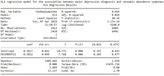
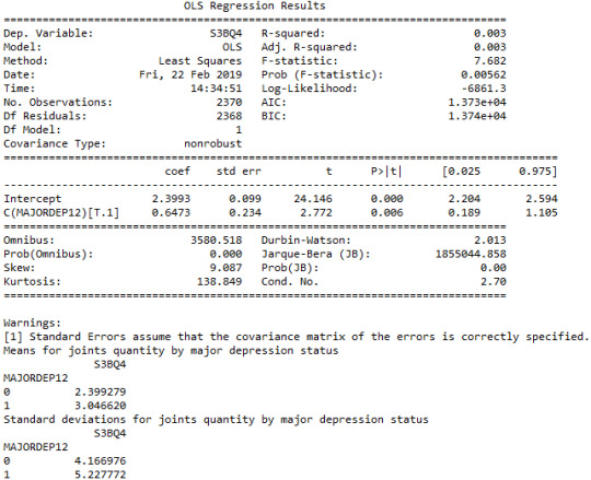
The linear regression model presented above aims to examine the association between major depression diagnosis in the last 12 months (categorical explanatory variable) and cannabis dependence symptoms (quantitative response variable), among U.S. adults aged between 18 and 30 years old. The number of observations that had valid data on both the response and explanatory variables and were therefore included in this analysis, was 2,412. The F-statistic is 60.34 and the P-value is 1.17e-14 (written in scientific notation). The P-value is considerably less than our alpha level of 0.05, which indicates that we can reject the null hypothesis and conclude that major depression diagnosis is significantly associated with cannabis dependence symptoms. In addition, the coefficient for major depression diagnosis is 0.38, and the intercept is 0.39. The P-value for our explanatory variable, in association with the response variable is p<0.0001 and the R-squared value, which is the proportion of the variance in cannabis dependence symptoms that can be explained by the major depression diagnosis, is significantly low at 2.4%.

Model Regression Equation

Bar Chart

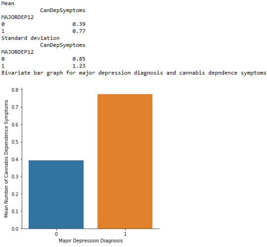
The bivariate bar graph presented above illustrates the association between major depression, diagnosed in the last 12 months (explanatory variable) and cannabis dependence symptoms (response variable), in U.S. adults aged from 18 to 30 years old. The “No” category of major depression diagnosis is coded with “0” and the “Yes” is coded with “1”. As we can see, the individuals diagnosed with major depression in the last 12 months appeared to have marginally double cannabis dependence symptoms (mean = 0.77), compared to those who did not meet the criteria for this disorder (mean = 0.39). Therefore, major depression diagnosis is significantly associated with cannabis dependence symptoms.

Exploring Statistical Interactions

This assignment aims to statistically assess the evidence, provided by NESARC codebook, in favour of or against the association between cannabis use and major depression, in U.S. adults. More specifically, I examined the statistical interaction between frequency of cannabis use (10-level categorical explanatory, variable ”S3BD5Q2E”) and major depression diagnosis in the last 12 months (categorical response, variable ”MAJORDEP12”), moderated by variable “S1Q231“ (categorical), which indicates the total number of the people who lost a family member or a close friend in the last 12 months. This effect is characterised statistically as an interaction, which is a third variable that affects the direction and/or the strength of the relationship between the explanatory and the response variable and help us understand the moderation. Since I have a categorical explanatory variable (frequency of cannabis use) and a categorical response variable (major depression), I ran a Chi-square Test of Independence (crosstab function) to examine the patterns of the association between them (C->C), by directly measuring the chi-square value and the p-value. In addition, in order visualise graphically this association, I used factorplot function (seaborn library) to produce a bivariate graph. Furthermore, in order to determine which frequency groups are different from the others, I performed a post hoc test, using Bonferroni Adjustment approach, since my explanatory variable has more than 2 levels. In the case of ten groups, I actually need to conduct 45 pair wise comparisons, but in fact I examined indicatively two and compared their p-values with the Bonferroni adjusted p-value, which is calculated by dividing p=0.05 by 45. By this way it is possible to identify the situations where null hypothesis can be safely rejected without making an excessive type 1 error.

Regarding the third variable, I examined if the fact that a family member or a close friend died in the last 12 months, moderates the significant association between cannabis use frequency and major depression diagnosis. Put it another way, is frequency of cannabis use related to major depression for each level of the moderating variable (1=Yes and 2=No), that is for those whose a family member or a close friend died in the last 12 months and for those whose they did not? Therefore, I set new data frames (sub1 and sub2) that include either individuals who fell into each category (Yes or No) and ran a Chi-square Test of Independence for each subgroup separately, measuring both chi-square values and p-values. Finally, with factorplot function (seaborn library) I created two bivariate line graphs, one for each level of the moderating variable, in order to visualise the differences and the effect of the moderator upon the statistical relationship between frequency of cannabis use and major depression diagnosis. For the code and the output I used Spyder (IDE).

Summary:

It seems that both the direction and the size of the relationship between frequency of cannabis use and major depression diagnosis in the last 12 months, is heavily affected by a death of a family member or a close friend in the same period. In other words, when the incident of a family/close death is present, the correlation is considerably weak, whereas when it is absent, the correlation is significantly strong and positive. Thus, the third variable moderates the association between cannabis use frequency and major depression diagnosis.

Hypothesis Testing and Pearson Correlation

This assignment aims to statistically assess the evidence, provided by NESARC codebook, in favor of or against the association between cannabis use and mental illnesses, such as major depression and general anxiety, in U.S. adults. More specifically, since my research question includes only categorical variables, I selected three new quantitative variables from the NESARC codebook. Therefore, I redefined my hypothesis and examined the correlation between the age when the individuals began using cannabis the most (quantitative explanatory, variable “S3BD5Q2F”) and the age when they experienced the first episode of major depression and general anxiety (quantitative response, variables “S4AQ6A” and ”S9Q6A”). As a result, in the first place, in order to visualize the association between cannabis use and both depression and anxiety episodes, I used seaborn library to produce a scatterplot for each disorder separately and interpreted the overall patterns, by describing the direction, as well as the form and the strength of the relationships. In addition, I ran Pearson correlation test (Q->Q) twice (once for each disorder) and measured the strength of the relationships between each pair of quantitative variables, by numerically generating both the correlation coefficients r and the associated p-values. For the code and the output I used Spyder (IDE).

The three quantitative variables that I used for my Pearson correlation tests are:

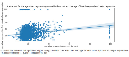
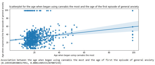
The scatterplot presented Below, illustrates the correlation between the age when individuals began using cannabis the most (quantitative explanatory variable) and the age when they experienced the first episode of depression (quantitative response variable). The direction of the relationship is positive (increasing), which means that an increase in the age of cannabis use is associated with an increase in the age of the first depression episode. In addition, since the points are scattered about a line, the relationship is linear. Regarding the strength of the relationship, from the Pearson correlation test we can see that the correlation coefficient is equal to 0.23, which indicates a weak linear relationship between the two quantitative variables. The associated p-value is equal to 2.27e-09 (p-value is written in scientific notation) and the fact that its is very small means that the relationship is statistically significant. As a result, the association between the age when began using cannabis the most and the age of the first depression episode is moderately weak, but it is highly unlikely that a relationship of this magnitude would be due to chance alone. Finally, by squaring the r, we can find the fraction of the variability of one variable that can be predicted by the other, which is fairly low at 0.05.

For the association between the age when individuals began using cannabis the most (quantitative explanatory variable) and the age when they experienced the first episode of anxiety (quantitative response variable), the scatterplot psented above shows a positive linear relationship. Regarding the strength of the relationship, the pearson correlation test indicates that the correlation coefficient is equal to 0.14, which is interpreted to a fairly weak linear relationship between the two quantitative variables. The associated p-value is equal to 0.0001, which means that the relationship is statistically significant. Therefore, the association between the age when began using cannabis the most and the age of the first anxiety episode is weak, but it is highly unlikely that a relationship of this magnitude would be due to chance alone. Finally, by squaring the r, we can find the fraction of the variability of one variable that can be predicted by the other, which is very low at 0.01.

Hypothesis Testing and Chi Square Test of Independence

cannabis users aged between 18 and 30 years old (subsetc2), my research question with the goal of generalizing the results to the larger population of NESARC survey, from where the sample has been drawn. Therefore, I statistically assessed the evidence, provided by NESARC codebook, in favor of or against the association between cannabis use and mental illnesses, such as major depression and general anxiety, in U.S. adults. As a result, in the first place I used crosstab function, in order to produce a contingency table of observed counts and percentages for each disorder separately. Next, I wanted to examine if the cannabis use status (1=Yes or 2=No) variable ‘S3BQ1A5’, which is a 2-level categorical explanatory variable, is correlated with depression (‘MAJORDEP12’) and anxiety (‘GENAXDX12’) disorders, which are both categorical response variables. Thus, I ran Chi-square Test of Independence (C->C) twice and calculated the χ-squared values and the associated p-values for each disorder, so that null and alternate hypothesis are specified. In addition, in order visualize the association between frequency of cannabis use and depression diagnosis, I used factorplot function to produce a bivariate graph. Furthermore, I used crosstab function once again and tested the association between the frequency of cannabis use (‘S3BD5Q2E’), which is a 10-level categorical explanatory variable, and major depression diagnosis, which is a categorical response variable. In this case, for my third Chi-square Test of Independence (C->C), after measuring the χ-square value and the p-value, in order to determine which frequency groups are different from the others, I performed a post hoc test, using Bonferroni Adjustment approach, since my explanatory variable has more than 2 levels. In the case of ten groups, I actually need to conduct 45 pair wise comparisons, but in fact I examined indicatively two and compared their p-values with the Bonferroni adjusted p-value, which is calculated by dividing p=0.05 by 45. By this way it is possible to identify the situations where null hypothesis can be safely rejected without making an excessive type 1 error. For the code and the output I used Spyder (IDE).

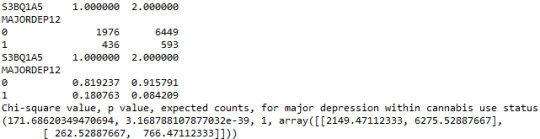
When examining the patterns of association between major depression (categorical response variable) and cannabis use status (categorical explanatory variable), a chi-square test of independence revealed that among young adults aged between 18 and 30 years old (subsetc1), those who were cannabis users, were more likely to have been diagnosed with major depression in the last 12 months (18%), compared to the non-users (8.4%), X2 =171.6, 1 df, p=3.16e-39 (p-value is written in scientific notation). As a result, since our p-value is extremely small, the data provides significant evidence against the null hypothesis. Thus, we reject the null hypothesis and accept the alternate hypothesis, which indicates that there is a positive correlation between cannabis use and depression diagnosis.

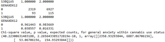
When testing the correlation between general anxiety (categorical response variable) and cannabis use status (categorical explanatory variable), a chi-square test of independence revealed that among young adults aged between 18 and 30 years old (subsetc1), those who were cannabis users, were more likely to have been diagnosed with general anxiety in the last 12 months (3.8%), compared to the non-users (1.6%), X2 =40.22, 1 df, p=2.26e-10 (p-value is written in scientific notation). As a result, since our p-value is again extremely small, the data provides significant evidence against the null hypothesis. Thus, we reject the null hypothesis and accept the alternate hypothesis, which indicates that there is a positive correlation between cannabis use and anxiety diagnosis.

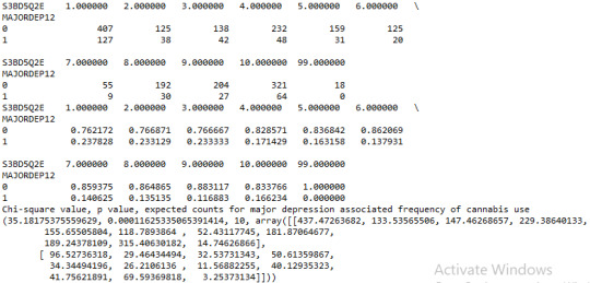
A Chi Square test of independence revealed that among cannabis users aged between 18 and 30 years old (subsetc2), the frequency of cannabis use (explanatory variable collapsed into 10 ordered categories) and past year depression diagnosis (response binary categorical variable) were significantly associated, X2 =35.18, 10 df, p=0.00011.

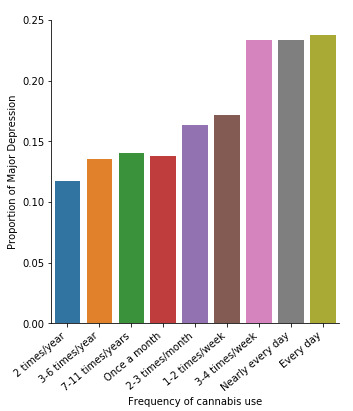
In the bivariate graph (C->C) presented above, we can see the correlation between frequency of cannabis use (explanatory variable) and major depression diagnosis in the past year (response variable). Obviously, we have a left-skewed distribution, which indicates that the more an individual (18-30) smoked cannabis, the better were the chances to have experienced depression in the last 12 months.

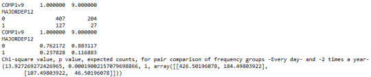
The post hoc comparison (Bonferroni Adjustment) of rates of major depression by the pair of “Every day” and “2 times a year” frequency categories, revealed that the p-value is 0.00019 and the percentages of major depression diagnosis for each frequency group are 23.7% and 11.6% respectively. As a result, since the p-value is smaller than the Bonferroni adjusted p-value (adj p-value = 0.05 / 45 = 0.0011>0.00019), we can assume that these two rates are significantly different from one another. Therefore, we reject the null hypothesis and accept the alternate.

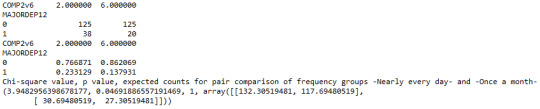
Similarly, the post hoc comparison (Bonferroni Adjustment) of rates of major depression by the pair of "Nearly every day” and “once a month” frequency categories, indicated that the p-value is 0.046 and the proportions of major depression diagnosis for each frequency group are 23.3% and 13.7% respectively. As a result, since the p-value is larger than the Bonferroni adjusted p-value (adj p-value = 0.05 / 45 = 0.0011<0.046), we can assume that these two rates are not significantly different from one another. Therefore, we accept the null hypothesis.

Hypothesis Testing and ANOVA

cannabis users aged between 18 and 30 years old (subsetc5), my research question with the goal of generalizing the results to the larger population of NESARC survey, from where the sample has been drawn. Therefore, I statistically assessed the evidence, provided by NESARC codebook, in favor of or against the association between cannabis use and mental illnesses, such as major depression and general anxiety, in U.S. adults. As a result, in the first place I used ols function in order to examine if depression (‘MAJORDEP12’) and anxiety ('GENAXDX12’) disorders, which are both categorical explanatory variables, are correlated with the quantity of joints smoked per day when using the most ('S3BQ4’), which is a quantitative response variable. Thus, I ran ANOVA (Analysis Of Variance) method (C->Q) twice and calculated the F-statistics and the associated p-values for each disorder separately, so that null and alternate hypothesis are specified. Furthermore, I used ols function once again and tested the association between the frequency of cannabis use ('S3BD5Q2E’), which is a 10-level categorical explanatory variable, and the quantity of joints smoked per day when using the most ('S3BQ4’), which is a quantitative response variable. In this case, for my third one-way ANOVA (C->Q), after measuring the F-statistic and the p-value, I used Tukey HSDT to perform a post hoc test, that conducts post hoc paired comparisons in the context of my ANOVA, since my explanatory variable has more than 2 levels. By this way it is possible to identify the situations where null hypothesis can be safely rejected without making an excessive type 1 error. In addition, both means and standard deviations of joints quantity response variable, were measured separately in each ANOVA, grouped by the explanatory variables (depression, anxiety and frequency of cannabis use) using the group by function. For the code and the output I used Spyder (IDE).

When examining the association between the number of joints smoked per day (quantitative response variable) and the past 12 months major depression diagnosis (categorical explanatory variable), an Analysis of Variance (ANOVA) revealed that among cannabis users aged between 18 and 30 years old (subsetc5), those diagnosed with major depression reported smoking slightly more joints per day (Mean=3.04, s.d. ±5.22) compared to those without major depression (Mean=2.39, s.d. ±4.16), F(1, 2368)=7.682, p=0.00562<0.05. As a result, since our p-value is extremely small, the data provides significant evidence against the null hypothesis. Thus, we reject the null hypothesis and accept the alternate hypothesis, which indicates that there is a positive correlation between depression diagnosis and quantity of joints smoked per day.

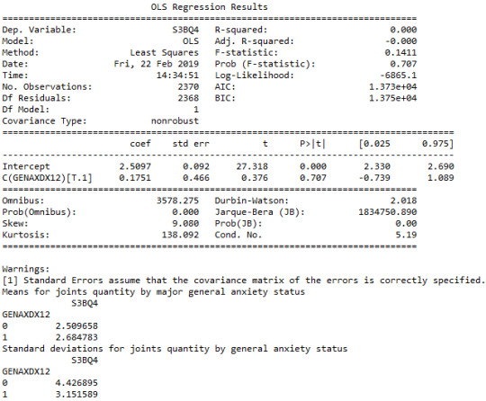
When testing the association between the number of joints smoked per day (quantitative response variable) and the past 12 months general anxiety diagnosis (categorical explanatory variable), an Analysis of Variance (ANOVA) revealed that among cannabis users aged between 18 and 30 years old (subsetc5), those diagnosed with general anxiety reported smoking marginally equal quantity of joints per day (Mean=2.68, s.d. ±3.15) compared to those without general anxiety (Mean=2.5, s.d. ±4.42), F(1, 2368)=0.1411, p=0.707>0.05. As a result, since our p-value is significantly large, in this case the data is not considered to be surprising enough when the null hypothesis is true. Consequently, there are not enough evidence to reject the null hypothesis and accept the alternate, thus there is no positive association between anxiety diagnosis and quantity of joints smoked per day.

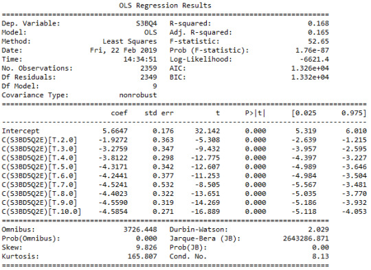
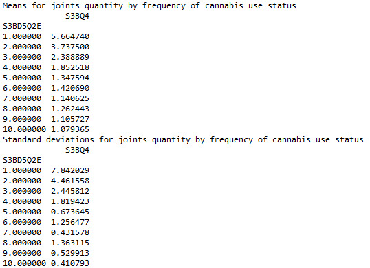
ANOVA revealed that among daily, cannabis users aged 18 to 30 years old (subsetc5), frequency of cannabis use (collapsed into 10 ordered categories, which is the categorical explanatory variable) and number of joints smoked per day (quantitative response variable) were relatively associated, F (9, 2349)=52.65, p=1.76e-87<0.05 (p value is written in scientific notation). Post hoc comparisons of mean number of joints smoked per day by pairs of cannabis use frequency categories, revealed that those individuals using cannabis every day (or nearly every day) reported smoking significantly more joints on average daily (every day: Mean=5.66, s.d. ±7.8, nearly every day: Mean=3.73, s.d. ±4.46) compared to those using 1 to 2 times per weak (Mean=1.85, s.d. ±1.81), or less. As a result, there are some pair cases in which using frequency and smoking quantity of cannabis, are positive correlated.

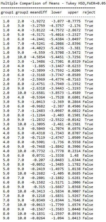
In order to conduct post hoc paired comparisons in the context of my ANOVA, examining the association between frequency of cannabis use and number of joints smoked per day when using the most, I used the Tukey HSD test. The table presented above, illustrates the differences in smoking quantity for each cannabis use frequency group and help us identify the comparisons in which we can reject the null hypothesis and accept the alternate, that is, in which reject equals true. In cases where reject equals false, rejecting the null hypothesis resulting in inflating a type 1 error.

Visualizing Data

In the final assignment are presented visualized data, taken from NESARC codebook, in order to examine the correlation between cannabis use and mental disorders such as major depression and general anxiety diagnosed in the last 12 months in a sample of 9535 U.S. young adults, aged from 18 to 30 years old. I used Spyder IDE to create both univariate and bivariate bar charts for the selected variables. More specifically, with variable ‘AGE’ between 18 and 30, I built unvariate graphs for categorical variables ‘S3BQ1A5’ which represents cannabis use, ‘S3BD5Q2E’ which is frequency of this use, ‘MAJORDEP12’ that stands for major depression diagnosis in the last 12 months and ‘GENAXDX12’ that indicates general anxiety diagnosis in the same period. In addition, you will find another univariate graph for the quantitative variable ‘NUMJOPMOTH_EST’, which I created in my previous assignment by multiplying frequency of cannabis use and average quantity of joints smoked, in order to estimate the total number of joints smoked per month by the individuals. As far as the bivariate graphs are concerned, I chose to examine visualized the association between cannabis use (C->C) and both mentioned disorders and additionally the relationship between frequency (C->C) and quantity (Q->C) of this use with both depression and anxiety. Thus, bar charts were created combining variables ‘S3BQ1A5’ (cannabis use), ‘S3BD5Q2E’ (frequency of use) and ‘NUMJOPMOTH_EST’ (quantity of joints) with variables ‘MAJORDEP12’ (major depression) and ‘GENAXDX12’ (general anxiety). Concluding, for the quantitative variable both center and spread were measured and describe function was used in order to examine useful information, about the selected categorical variables.

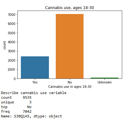
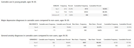
A random sample of 9535 U.S. young adults, aged 18-30, were asked, as a part of NESARC survey, the following question: “Have you ever used cannabis?” A percentage of 25.29% (or 7042 individuals) answered “Yes”, whereas 73.85% (or about 2500 individuals) answered “No” which was the most frequent answer. Also a significantly small percentage of 0.84%, fell into category 9 (“Unknown“) which is our missing data.

To the question of “How often did you use cannabis when using the most?”, the top answer was “Every day”, since 534 individuals fell into this category, followed by “Once a year” category with approximately 400 individuals. Less than 100 people chose “7-11 times per year” category, which was the least frequent answer.

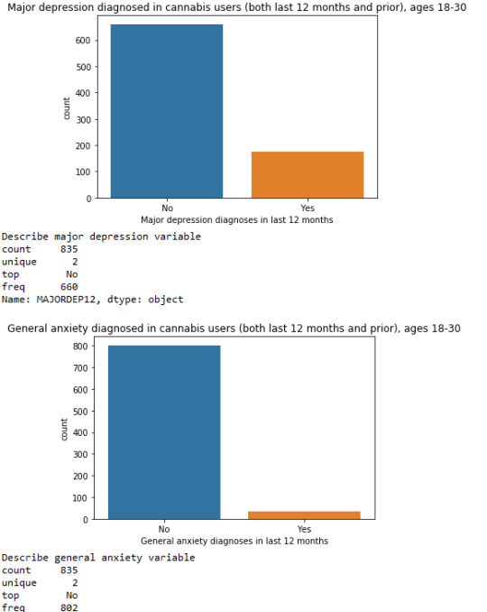
Of the total number of participants (18-30) who answered “Yes” to the question of cannabis use, only those who were smoking marijuana in last 12 months and prior were taken into consideration for the next two questions.

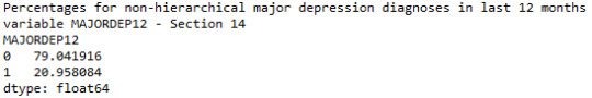
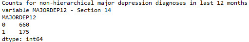
To the question of “Have you been diagnosed with non-hierarchical major depression in the last 12 months?”, about 660 participants or 79.04% answered “No” which was the most frequent answer, whereas 175 or 20.95% fell into “Yes”.

For the question, ”Have you been diagnosed with non-hierarchical generalized anxiety in the last 12 months?”, 802 individuals or 96.04% answered “No“ that was our top answer, while only 33 or 3.95% chose “Yes“.

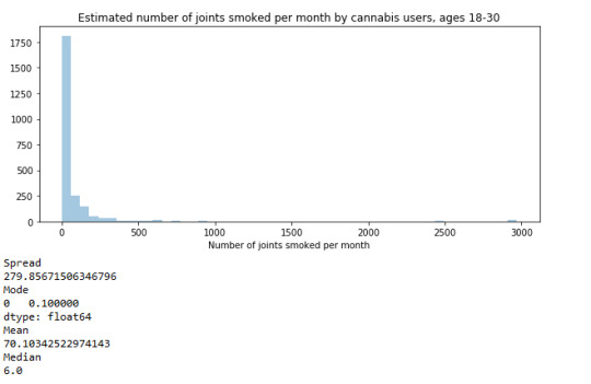
For the estimated number of joints smoked per month by cannabis users, ages 18-30, it noticeable from the graph that there was a skewed-right distribution. The spread or the standard deviation of the variable is extremely large which indicates a large variety of answers among the participants. The three main numerical measures of the center of the distribution are the mode, the median, and the mean. Here we can see that mode is equal to 0.1 and it was the most common occurring value in the distribution, which means that most of participants smoked less than 1 joint per month. The mean is equal to 70.1 which indicates that cannabis users smoked about 70 joints per month on average and the median or the middle value is 6.

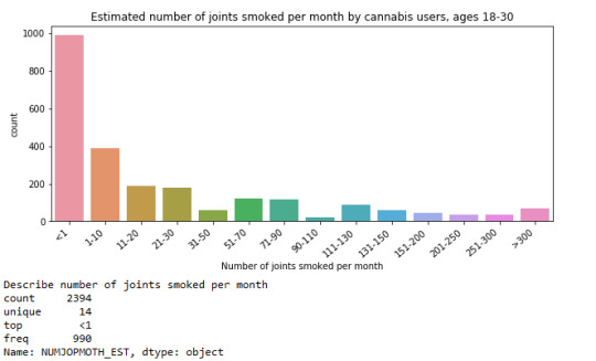
Estimated number of joints smoked per month binned to groups as illustrated above. Another way of visualizing the distribution of variable ‘NUMJOPMOTH_EST’. We can see that most individuals, about 990, smoked less than one joint per month and the shape of the distribution is right-skewed.

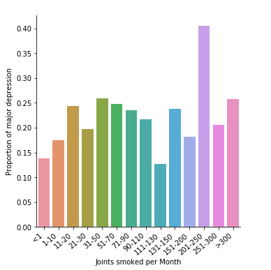
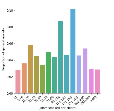
In the bar charts above we can see the relationship between quantity of joints smoked per month by cannabis user, aged 18 to 30 years old, and both major depression (first) and general anxiety (second) diagnoses in the last 12 months (Q->C). The explanatory variable is quantity of joints (quantitative), while the response variables are depression and anxiety diagnoses (categorical). There is a slightly increasing trend in the first graph, but not in the second.

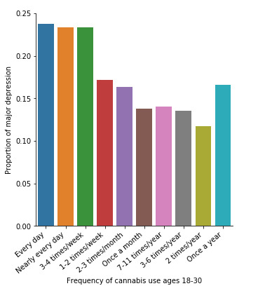
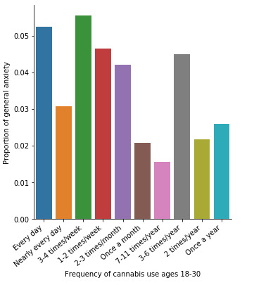
In the graphs presented above we can see the correlation between frequency of cannabis use and both major depression and general anxiety (C->C). The explanatory variable is frequency of cannabis use (categorical), while the response variables are depression and anxiety diagnoses (categorical). Again, for the first graph we have a right-skewed distribution, which indicates that the more an individual smoked cannabis, the better were the chances to get diagnosed with depression. However, we cannot support the same as far as anxiety is concerned, which appears to have a more raffle and abnormal distribution.

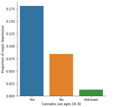
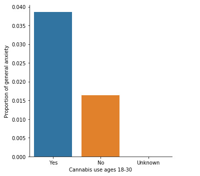
To sum up, looking through the the last graphs, it can be noticed that there are some slight differences between the percentages of cannabis users compared to non-users. Major depression cases in cannabis users young adults (20.95%) seem to be slightly more than double compared to those of non-users (8.42%).In addition, general anxiety diagnoses in cannabis users (3.95%) appear to be also marginally more than double in comparison to the non-users (1.63%). It could be supported that there is a relative association between cannabis and such mental disorders, thus cannabis use increases the likelihood of meeting criteria for depression or general anxiety in the future. However, the sample is extremely small and it is unclear how representative it is, making the findings less reliable, since a large amount of error may be involved.

Making Data Management Decisions

In this assignment you will find three data managed variables, provided from NESARC codebook, as frequency distributions. For the variable ‘AGE’, I decided to split the ages of the observations in four categories (18-21, 21-24, 24-27, 27-30), in order to examine the age frequency distribution of the sample into quartiles. Furthermore, I included missing data in the cannabis use variable distribution for ages 18 to 30, with the row ‘Unknown’ set to ‘nan’. In addition, after recoding variable ‘S3BD5Q2E’, which represents average rate of cannabis use, I created a new variable called ‘CUFREQMO’ that indicates how many days an individual used cannabis per month, when using the most. Moreover, once I ran frequency distribution for the variable ‘CUFREQMO’ and calculated the counts and the percentages of this use per month, I created a secondary variable with the name ‘NUMJOPMOTH_EST’. This variable estimates the quantity of cannabis joints smoked per month for the first 30 participants (18-30) when using the most, by multiplying the amount of joints smoked per day (variable ‘S3BQ4’) with the variable ‘CUFREQMO’, which indicates the number of days an individual smoked per month. I finished with the creation of one more variable called ‘NUMMDGENANX’ that stands for the total number of participants who were diagnosed with either major depression, general anxiety or both illnesses. After examining the frequency distribution of this variable, I used the define function to create one last variable with the name ‘DEPRESSIONANXIETY’, which characterizes the mental state of the first 30 random cannabis users aged 18 to 30, as far as these two disorders are concerned. For the code and the output i used Spyder (IDE).

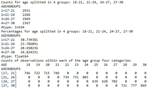
Firstly, a new variable called ‘AGE4GROUPS’ was necessary to be created in order to divide participants, aged between 18 and 30 years old, into four age groups: 18-21, 21-24, 24-27 and 27-30. From the frequency distribution it can be noticed that about 30.73% were between 18 and 21 years old, 23.78% were between 21 and 24, 20.65% fell into 24-27 group and 24.82% fell into 27-30 group.

For the frequency distribution of variable ‘S3BQ1A5′ the missing data is included and option 9 is set to ‘NaN’, which represents the choice ‘Unknown’. As we can see the number of the missing data is 81 individuals and the proportion is 0.84% which is significantly small. Regarding the new variable with the name ’CUFREQMO’ which I created, the distribution results show that about 15.96% smoked cannabis less than once per year, whereas approximately 22.13% used to smoke cannabis in an everyday basis. The rest of the cannabis use rates vary from about 2.65% for less than once per month, to 11.6% for an average use of 6 times per month.

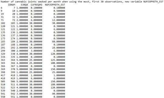
Taking into account the new variable ‘NUMJOPMOTH_EST’ which I created, the output illustrates the estimation of the quantity of joints smoked by young adults aged 18 to 30 per month, by multiplying the quantity of joints smoked per day with the total number of days that they used cannabis per month. By examining the first 30 observations of the sample, it is noticeable that the majority of individuals smoked approximately less than 10 joints per month. On the other hand there were also some participants who were smoking more than 100 joints monthly, since individuals with ID numbers 511 and 506 for example, peaked at 180 and 150 joints per month respectively.

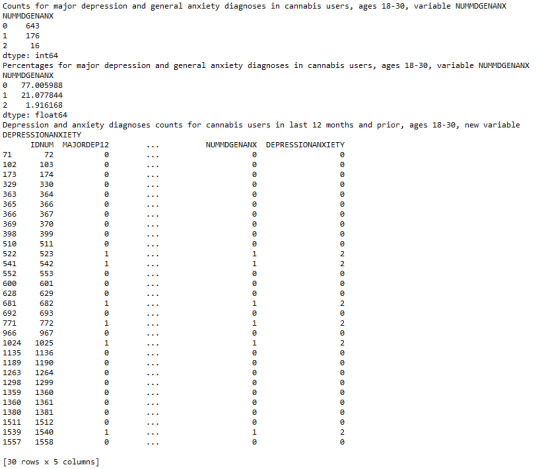
As far as the new secondary variable ‘NUMMDGENANX’ is concerned, it is obvious that around 77% of cannabis users aged between 18 and 30 were mentally healthy in the last 12 months, after using marijuana for more than 1 year, while a percentage of 21.07% were diagnosed with either major depression or general anxiety. Only 1.91% of them were diagnosed with both mental disorders mentioned above. Finally, regarding the first 30 observations table, presented in the end, the define function used, returns 0 if an individual had no problem with either depression or anxiety in the last 12 months, 1 if an individual met the criteria for both disorders, 2 if an individual was diagnosed only with major depression and 3 if an individual was diagnosed only with general anxiety. For the results, a new variable named ‘DEPRESSIONANXIETY’ was created.

Writing my first program - Python

In order to examine frequency distributions for my selected variables, I chose to use Spyder, a python integrated development environment (IDE). Once I have run frequency distributions for all of my chosen variables, I decided to subset my dataset and ask my question based on a specific set of observations, instead of the entire sample. I found myself most interested in the association between cannabis use and major depression as well as general anxiety disorders diagnosed in the last 12 months, but only among young adults between 18 and 30 years old who have used cannabis both in last 12 months and before. Moreover, the results of the subset mentioned above will be compared with the outcomes of my secondary subset, which aims to examine the same association, but this time only among young adults, aged 18-30, who have never used cannabis. Finally, a general proportion of cannabis use among adults between 18 and 30 years old, will also be presented.

Subset1

For the variable ‘AGE’ I decided to include two logic statements which are particular rows in the NESARC dataset. These are [‘AGE’]>=18 and ['AGE’]<=30. In addition, as far as variable 'S3BQ1A5’ is concerned, which represents cannabis use, the logic statement ['S3BQ1A5’]==1 (1=Yes) should also be included. Finally, for the variable 'S3BD5Q2B’ that represents the period of the use, only the row ['S3BD5Q2B’]==3 (3=During both time periods) was taken into account.

Subset2

Same as subset1, the logic statements for variable ‘AGE’ are ['AGE’]>=18 and ['AGE’]<=30. Alternatively in this case, since we need to examine the results among only non-users young adults, the logic statement for cannabis use variable 'S3BQ1A5’ is ['S3BQ1A5’]==2 (2=No).

Report

A random sample of 9535 U.S. young adults, aged 18-30, were asked, as a part of NESARC survey, the following question: “Have you ever used cannabis?” A percentage of 25.29% answered “Yes”, whereas 73.85% answered “No”. Also a significantly small percentage of 0.84%, fell into category 9 (“Unknown“) which is our missing data.

Of the total number of participants (18-30) who answered “Yes” to the question of cannabis use, only those who were smoking marijuana in last 12 months and prior were taken into consideration for the next questions.

To the question of “Have you been diagnosed with non-hierarchical major depression in the last 12 months?”, about 20.95% of the cannabis users responded “Yes” while only 8.42% of the non-users answered the same.

For the question, ”Have you been diagnosed with non-hierarchical generalized anxiety in the last 12 months?”, a proportion of 3.95% of cannabis users were diagnosed positive to anxiety disorders compared to 1.63% of the non-users.

Conclusion

To sum up, looking through the the frequency table it can be noticed that there are some slight differences between the percentages of cannabis users compared to non-users. Major depression cases in cannabis users young adults (20.95%) seem to be slightly more than double compared to those of non-users (8.42%).In addition, general anxiety diagnoses in cannabis users (3.95%) appear to be also marginally more than double in comparison to the non-users (1.63%). It could be supported that there is a relative association between cannabis and such mental disorders, thus cannabis use increases the likelihood of meeting criteria for depression or general anxiety in the future. However, the sample is extremely small and it is unclear how representative it is, making the findings less reliable, since a large amount of error may be involved.

Introduction

After reviewing the codebook of NESARC, a survey in over 43093 U.S. citizens (over the age of 18) designed to determine the magnitude of alcohol use and psychiatric disorders, I found myself particularly interested in cannabis use disorders. More specifically I aim to examine the patterns of association between cannabis use, and major depression as well as general anxiety disorder diagnosed in the last 12 months. Nowadays, cannabis is the most widely consumed drug in many countries, however there is also a medical use of it. It has been estimated that around 10% of people who use cannabis will become depended upon it [4]. It is common knowledge that there is a strong relationship between mental disorders and alcohol abuse, therefore it is a matter of interest whether cannabis’ frequent use co-occurs with depression and generalized anxiety.

Research Question

Is cannabis use associated with major depression and general anxiety disorder diagnoses in the last 12 months?

Hypothesis

Despite the fact that several studies have examined issues relevant to cannabis abuse disorders, its difficult to decide if cannabis use leads to psychiatric illnesses. At this point it is necessary to separate cannabis use from a heavier involvement with the drug (dependence / abuse). My personal belief is that cannabis use increases the likelihood of depression symptoms and anxiety disorders, however not as significantly as cannabis abuse / dependence, which could cause mental disorders like the ones mentioned above.

NESARC Codebook Sections and Variables

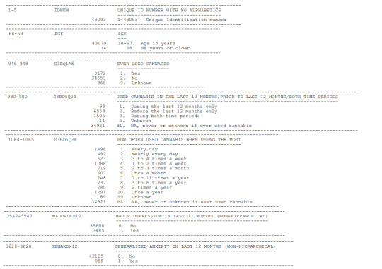
After looking through NESARC codebook, firstly i decided to take into consideration the unique identification number (IDNUM) and the variable (AGE) from background information (SECTION 1) of the sample, in order to make my findings more reliable. Furthermore for my first question topic I chose, from the drug / medicine use section (SECTION 3B), to include information like the percentage of people who ever used cannabis (S3BQ1A5), as well as the period of this use -last 12 months / prior to last 12 months / both periods- (S3BD5Q2B) and the frequency of it when using the most (S3BD5Q2E). As far as the second topic is concerned, I selected the variable of non-hierarchical major depression diagnosis, in last 12 months (MAJORDEP12) and the variable of non-hierarchical generalized anxiety diagnosis, in last 12 months (GENAXDX12), which are included in the diagnoses section (SECTION 14).