fanalyst - Tumblr blog

fanalyst · 7 years

Text

Random Forest!

In this post, I show how I applied a random forest to find the significance of three explanatory variables on my binary target variable. My target variable is whether or not adolescent students had to repeat a grade or were held back a grade at school (0=no, 1=yes). The three explanatory variables I studied were the paternal presence (0=no dad, 1= dad present), the maternal presence (0=no mom, 1= mom present), and self-assessed health status (0=bad health, 1= any other response). Below is the python output of my random forest model:

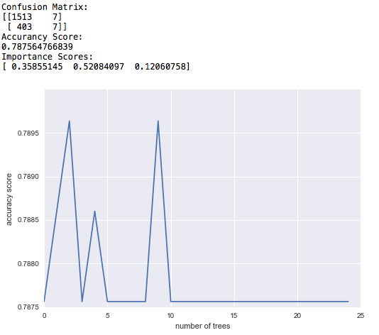
As indicated by the accuracy score, the model can predict the right response about 79% of the times when 25 trees are used.

The importance scores tell us which of the variables are more significant in predicting the target variable. In this case, the paternal presence is the most significant variable (IS=0.52). The health status comes in the second place (SI=0.36) and maternal presence is the least significant of all three (IS=0.12).

The graph shows how the accuracy score changes as the number of trees used in the model increases. As we can see, for the number of trees from 1 to 25, the results do not change much and in any case, the accuracy score is about 0.79. Though the score converges after 10 trees.

My Python code:

# -*- coding: utf-8 -*- """ Created on Fri Dec 23 22:18:49 2016

@author: Farshad """

#load the packages import pandas import numpy import seaborn import matplotlib.pyplot as plt import statsmodels.formula.api as smf import statsmodels.stats.multicomp as multi import scipy.stats import itertools import statsmodels.api as sm from sklearn.cross_validation import train_test_split from sklearn.tree import DecisionTreeClassifier from sklearn.metrics import classification_report from sklearn.ensemble import RandomForestClassifier import sklearn.metrics #call data data=pandas.read_csv('addhealth_pds.csv',low_memory=False) # set pandas to show all columns and rows in dataframe pandas.set_option('display.max_columns',None) pandas.set_option('display.max_rows',None)

print(len(data)) # number of individuals print(len(data.columns)) # number of variables

#upper-case all the DataFrame column names data.columns=map(str.upper, data.columns)

#bug fix for display formats to avoid run time errors pandas.set_option('display.float_format', lambda x: '%f' %x)

#covert values to numerics... This avoids issues with ordering of values data["H1ED5"]=pandas.to_numeric(data["H1ED5"], errors='coerce') data["H1ED11"]=pandas.to_numeric(data["H1ED11"], errors='coerce') data["H1ED12"]=pandas.to_numeric(data["H1ED12"], errors='coerce') data["H1ED13"]=pandas.to_numeric(data["H1ED13"], errors='coerce') data["H1ED14"]=pandas.to_numeric(data["H1ED14"], errors='coerce') data["H1WP13"]=pandas.to_numeric(data["H1WP13"], errors='coerce') data["H1WP9"]=pandas.to_numeric(data["H1WP9"], errors='coerce') data["H1ED14"]=pandas.to_numeric(data["H1ED14"], errors='coerce') data["BIO_SEX"]=pandas.to_numeric(data["BIO_SEX"], errors='coerce') data["H1GH1"]=pandas.to_numeric(data["H1GH1"], errors='coerce') data["AGE"]=pandas.to_numeric(data["AGE"], errors='coerce')

recode3={1:1, 2:1, 3:1, 4:0, 5:0, 6:numpy.nan, 7:numpy.nan} data['HLTH']=data['H1GH1'].map(recode3) recode2={1:1, 2:1, 3:1, 4:1, 5:1, 6: numpy.nan, 7: 0, 8: numpy.nan} #7: non dad data['DAD']=data["H1WP13"].map(recode2) data['MOM']=data["H1WP9"].map(recode2) data["BIO_SEX"]=data["BIO_SEX"].replace(6,numpy.nan) data['BIO_SEX']=data['BIO_SEX'].replace(2, 0) data["H1ED5"]=data["H1ED5"].replace([6,8],numpy.nan) data_clean=data.dropna() data_clean.dtypes data_clean.describe()

predictors=data_clean[['HLTH','DAD','MOM']] targets=data_clean.H1ED5

pred_train, pred_test, tar_train, tar_test = train_test_split(predictors, targets, test_size=.4) pred_train.shape pred_test.shape tar_train.shape tar_test.shape

#Build model on training data classifier=RandomForestClassifier(n_estimators=25) classifier=classifier.fit(pred_train,tar_train)

predictions=classifier.predict(pred_test)

print('Confusion Matrix:') print(sklearn.metrics.confusion_matrix(tar_test,predictions)) print('Accurancy Score:') print(sklearn.metrics.accuracy_score(tar_test, predictions))

model=sklearn.ensemble.ExtraTreesClassifier() model.fit(pred_train,tar_train) print('Importance Scores:') print(model.feature_importances_) trees=range(25) accuracy=numpy.zeros(25) for idx in range(len(trees)): classifier=RandomForestClassifier(n_estimators=idx+1) classifier=classifier.fit(pred_train,tar_train) predictions=classifier.predict(pred_test) accuracy[idx]=sklearn.metrics.accuracy_score(tar_test,predictions)

plt.cla() plt.plot(trees,accuracy) plt.xlabel('number of trees') plt.ylabel('accuracy score')

0 notes

fanalyst · 7 years

Text

A simple classification tree:

I ran a decision tree to find the contribution of three categorical explanatory variables to whether or not student adolescents have to repeat a grade at school (binary categorical target variable). The predictive variables I chose for this model are:

MOM: the maternal presence (0= no mom, 1= have a mom)

DAD: the paternal presence (0=no dad, 1= have a dad)

HLTH: self-assessed state of health (0= bad health 1= every other response)

Below are the confusion matrix and the accuracy score of the model:

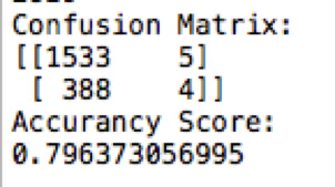
So the model is accurate about 80% of the times. And the decision tree:

From the decision tree, we can see that those adolescents who had neither of their parents present and reported bad health are most likely to be held back a grade at school. On the other hand, those that had both parents present and did not report a bad health condition were least likely to be held back a grade (not too surprising ha?).

Adding more explanatory variables or quantitative variables drastically increases the size of the tree.

Python code for this analysis: (the code was required to be copy and pasted; sorry for the lack of readability)

# -*- coding: utf-8 -*- """ Created on Fri Dec 23 22:18:49 2016

@author: Farshad """

#load the packages import pandas import numpy import seaborn import matplotlib.pyplot as plt import statsmodels.formula.api as smf import statsmodels.stats.multicomp as multi import scipy.stats import itertools import statsmodels.api as sm from sklearn.cross_validation import train_test_split from sklearn.tree import DecisionTreeClassifier from sklearn.metrics import classification_report import sklearn.metrics #call data data=pandas.read_csv('addhealth_pds.csv',low_memory=False) # set pandas to show all columns and rows in dataframe pandas.set_option('display.max_columns',None) pandas.set_option('display.max_rows',None)

print(len(data)) # number of individuals print(len(data.columns)) # number of variables

#upper-case all the DataFrame column names data.columns=map(str.upper, data.columns)

#bug fix for display formats to avoid run time errors pandas.set_option('display.float_format', lambda x: '%f' %x)

predictors=data_clean[['HLTH','DAD','MOM']] targets=data_clean.H1ED5

pred_train, pred_test, tar_train, tar_test = train_test_split(predictors, targets, test_size=.4) pred_train.shape pred_test.shape tar_train.shape tar_test.shape

#Build model on training data classifier=DecisionTreeClassifier(max_depth=6) classifier=classifier.fit(pred_train,tar_train)

predictions=classifier.predict(pred_test)

print('Confusion Matrix:') print(sklearn.metrics.confusion_matrix(tar_test,predictions)) print('Accurancy Score:') print(sklearn.metrics.accuracy_score(tar_test, predictions))

#Displaying the decision tree from sklearn import tree #from StringIO import StringIO from io import StringIO #from StringIO import StringIO from IPython.display import Image out = StringIO() tree.export_graphviz(classifier, out_file=out,feature_names=['HLTH','DAD','MOM']) import pydotplus graph=pydotplus.graph_from_dot_data(out.getvalue()) #Image(graph.create_png()) with open('picture_out1.png', 'wb') as f: f.write(graph.create_png())

0 notes

fanalyst · 7 years

Text

A logistic regression model:

Suppose that we are interested in knowing the effects of several explanatory variables on the odds of the adolescents having to repeat a grade or being held back a grade at school. In this case, the response variable is binary so we need a logistic regression model. The response variables are: The paternal presence (0=no dad, 1= dad present), the maternal presence (0= no mom, 1= mom present), self-assessed health status (0=bad health, 1=every other response), and biological sex (0= female, 1=male).

Here’s the output of my python code for the logistic regression model:

The analysis shows that all the aforementioned variables are statistically significant (p<0.001) and there is no indication of presence of confounding variables (among those that were investigated). However, the pseudo-r-square is only about 0.04, which means that the model can explain only 4% of the variability in the values of the explanatory variable. This signals to the fact that the model does not include some important predictive variables.

We can better analyse our findings by looking at odd ratios and confidence intervals for the odd ratios:

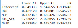
We can draw the following conclusions:

1- When controlling other response variables, the odds of the adolescents having to repeat a grade (or being held back a grade) is about 1.8 times higher for those that do not have a father comparing to those that have a father (OR= 0.54, 95% CL=[0.481- 0.619], p<0.001) .

2- When controlling other response variables, the odds of the adolescents having to repeat a grade (or being held back a grade) is about 1.8 times higher for those that do not have a mother comparing to those that have a mother (OR= 0.54, 95% CL=[ 0.432-0.686], p<0.001) .

3- When controlling other response variables, the odds of the adolescents having to repeat a grade (or being held back a grade) is about 1.8 times higher for boys that girls (OR= 1.79, 95% CL=[ 1.586-2.028], p<0.001) .

4- When controlling other response variables, the odds of the adolescents having to repeat a grade (or being held back a grade) is about 2.3 times higher for those adolescents who believed that they were not healthy comparing to others (OR= 0.44, 95% CL=[ 0.354 0.540], p<0.001) .

My Python Code for this analysis:

0 notes

fanalyst · 7 years

Text

A multivariable regression model…

Here I want to investigate the association between several explanatory variables and the adolescents’ estimated GPA (quantitative variable). The explanatory variables that I consider are: age (quantitative, centered around 0), biological sex (categorical binary, F=0, M=1), paternal presence (categorical binary, 0=no dad), maternal presence (categorical binary, 0=no mom), self-assessed state of health (categorical binary, 0=bad health, 1= OK or good health).

Then I ran a multivariable regression model of these variables.

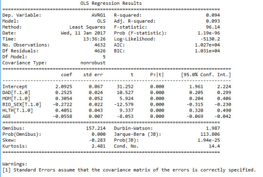
The R-squared value is about 0.1 which means that the model can explain only 10% of the variation in the response variable. The p-value of all the explanatory variables are very small (p<0.001), hinting that all the associations are statistically significant (though weak overall). The following linear predictive function can be suggested based on the results:

GPA=2.1+0.25*DAD+0.30*MOM-0.27*BIO_SEX+0.40*HLTH-0.05*AGE

For the paternal presence, the parameter estimate is 0.25 and the confidence interval for the population is [0.205 0.299]. For the maternal presence, the parameter estimate is 0.30 and the confidence interval for the population is [0.204 0.406]. For the biological sex, the parameter estimate is -0.27 (negative association) and the confidence interval for the population is [-0.315 -0.230]. For the self-assessed health status, the parameter estimate is 0.40 and the confidence interval for the population is [0.320 0.490]. And finally, for age, the parameter estimate is -0.05 (negative association) and the confidence interval for the population is [-0.069 -0.042]. There is no evidence of nay confounding variables (among those investigated) since all the p-values are very small.

Below is the quantile-quantile plot for the model:

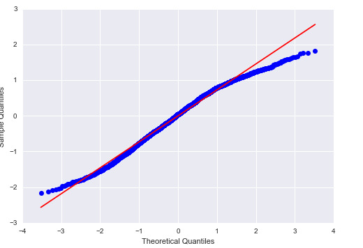
For the most part, the actual residuals follow the same pattern as the predicted (normal) residuals; however, there are some deviations from it for low and high values of quantiles, hence the model is not perfect.

The normalized residual plot for this model is presented below:

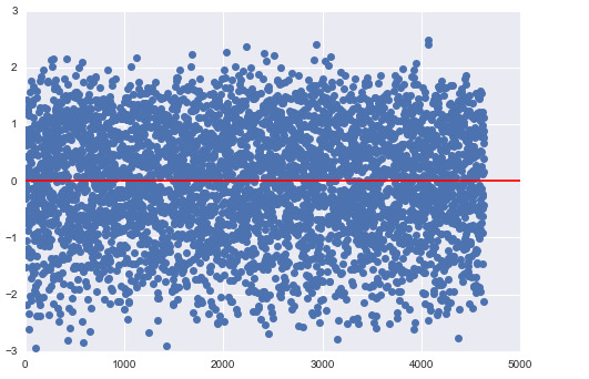
We see quite a few data points that are above 2*std and below -2*std, which shows that there is appreciable error involved in the model. This could be due to neglecting other important explanatory variables that are not included in the current model.

We can also look at some diagnostic graphs. Here, I am showing these plots for the variable, AGE:

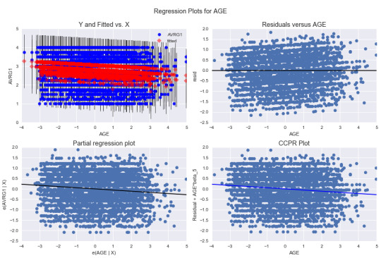
The top right plot shows the residual versus age. The residuals seem to be randomly distributed, but the graph points out to some outliers.

The bottom left plot is the partial regression plot which shows the effect of age on GPA when controlling other variables. The plot shows the weak negative association between age and GPA.

Finally, let’s look at the leverage plot for this regression model:

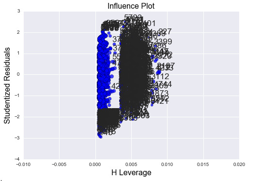
The plot shows that most of the data have very low H-leverage (<0.005), but some of the data are further away to the right. Most of the outliers are on the lower end of the H-value, which means that they do not affect the model much, but there are some outliers that have relatively higher H-value. However, we do not have any outliers that are greater over 2.5*std or under -2.5*std.

The Python code for this analysis:

Note: I’d like to thank everyone for their constructive comments. I decided to add images of my code rather than the actual scripts in order to improve readability.

0 notes

fanalyst · 7 years

Text

A univariate regression model

Here, I want to find out if there is an association between the GPA of the adolescents and having or not having a father. The explanatory variable is the paternal presence (having or not having a father) and response variable is the estimated unweighted GPA of the adolescents (1-4). Below is the frequency distribution for the explanatory variable (DAD):

Since the explanatory variable is binary categorical, I prepare the variable such that the value 0 correspond to the state of not having a father and value 1 to correspond to the state of having a father. Figure below shows the bivariate bar chart for the correlation between the GPA and paternal presence.

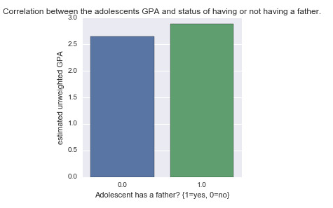
It shows that those in the 1 category have higher mean value of GPA than those in the 0 category. We can run a simple regression model to investigate the significance and strength of this association.

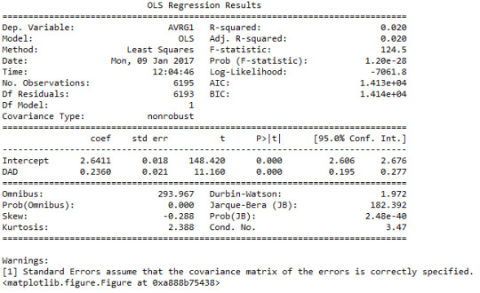
We see that p-value is very small (<0.001) so the association is meaningful, but the r-squared value is 0.02 which means that only 2 percent of the variation in the response variable can be explained using this explanatory variable. Hence the correlation is weak, but significant. This means that we need other additional explanatory variables to explain the variations in the response variable. Since the parameter estimate is positive (beta_1=0.2360), the correlation is a positive correlation. Based on the current regression model, we can suggest the following correlation between the two variables:

Y=2.6411+0.236*x,

where x is the paternal presence (0,1) and y is the estimated unweighted GPA (1-4). Note that if we substitute values of 0 and 1 for the x variable we get the mean values of GPA for the two categories: 2.64 and 2.87 respectively. These are in agreement with the findings from the bivariate bar chart above.

My Python code for this post:

# -*- coding: utf-8 -*- """ Created on Fri Dec 23 22:18:49 2016

@author: Farshad """

#load the packages import pandas import numpy import seaborn import matplotlib.pyplot as plt import statsmodels.formula.api as smf import statsmodels.stats.multicomp as multi import scipy.stats import itertools #call data data=pandas.read_csv('addhealth_pds.csv',low_memory=False) # set pandas to show all columns and rows in dataframe pandas.set_option('display.max_columns',None) pandas.set_option('display.max_rows',None)

print(len(data)) # number of individuals print(len(data.columns)) # number of variables

#upper-case all the DataFrame column names data.columns=map(str.upper, data.columns)

#bug fix for display formats to avoid run time errors pandas.set_option('display.float_format', lambda x: '%f' %x)

#data["H1ED7"]=data["H1ED7"].astype(numpy.int64) #calculate and print count values. drpna displays the values that are missing using NaN.

recode1={1:4, 2:3, 3:2, 4:1, 5:99, 96:numpy.nan, 97:99, 98:numpy.nan} # dummy 99 is when the student didn't take the course or had legitimate skip data['MATH1']=data["H1ED12"].map(recode1) data['ENGL1']=data["H1ED11"].map(recode1) data['SCIE1']=data["H1ED14"].map(recode1) data['HIST1']=data["H1ED13"].map(recode1) def AVRG1 (row): if numpy.isnan(row['MATH1']) or numpy.isnan(row['ENGL1']) or numpy.isnan(row['SCIE1']) or numpy.isnan(row['HIST1']): return numpy.nan else: i=(row['MATH1']==99)+(row['ENGL1']==99)+(row['SCIE1']==99)+(row['HIST1']==99) if i==4: return numpy.nan else: return ((row['MATH1']!=99)*row['MATH1']+(row['ENGL1']!=99)*row['ENGL1']+(row['SCIE1']!=99)*row['SCIE1']+(row['HIST1']!=99)*row['HIST1'])/(4-i) data['AVRG1']=data.apply(lambda row: AVRG1(row),axis=1)

data['AVRG%']=pandas.qcut(data.AVRG1, 5, labels=["bottom20%", "bottom40%", "middle20%", "top40%", "top20%"])

recode2={1:1, 2:1, 3:1, 4:1, 5:1, 6: numpy.nan, 7: 0, 8: numpy.nan} #7: non dad data['DAD']=data["H1WP13"].map(recode2)

print('percentage of DAD: (MANAGED) Do the adolescents have a father? {1=yes, 0=no}') p11=data["DAD"].value_counts(sort=False, normalize=True, dropna=False)*100 print(p11.sort_index())

''' #rename categories data["DAD"]=data["DAD"].astype('category') print('Summary statistics of DAD: Do the adolescents have a father? {1=yes, 0=no}') desc3=data['DAD'].describe() print(desc3) '''

#bivariate bar chart plt.figure() seaborn.factorplot(x='DAD',y='AVRG1', data=data, kind="bar", ci=None) plt.xlabel('Adolescent has a father? {1=yes, 0=no}') plt.ylabel('estimated unweighted GPA') plt.title('Correlation between the adolescents GPA and status of having or not having a father.') sub1=data[['AVRG1','DAD']].dropna() # model1=smf.ols(formula='AVRG1 ~ DAD', data=sub1).fit() print(model1.summary())

0 notes

fanalyst · 7 years

Text

A little bit about the data:

Sample: The sample used in this analysis is made available by the first wave of the National Longitudinal Study of Adolescent to Adult Health (Add Health) survey. This survey is based on school-sampling of 80 high schools in the United States during 1994-1995. The selection of schools is done using implicit stratification, assuring true representation of US high school with respect to region, urbanity, size, type and ethnicity. All of these schools included 11th grade and enrolled more than 30 students. The participating schools, also, helped to identify other feeder schools, providing a total of 132 schools. The participants in this study are N=90,000 adolescent individuals in 7-12 grades.

Procedure: The survey studies N=90,000 adolescents in grade 7-12 using in-class questionnaires that were self-administered and formatted for optical scanning. The questionnaires were administered in 50-60 minute sessions between September 1994 and April 1995 and was performed to investigate adolescents’ heath and risky behavior. It encompassed topics including family, school, and communities.

Measure: As the response variable, we obtain an estimate of unweighted GPA of the adolescents from the self-reported grades for 4 subjects: English, mathematics, history, and science. This was done by converting the categorical letter-grade variables to quantitative grades and finding unweighted average of the four subjects for each individual (aggregating 4 variables). This variable can obtain continuous values between 1 and 4. We are also interested in the level of closeness of the adolescents to their fathers (as the explanatory variable). This was measured through the answer to the question: “How close do you feel to your Father/Stepfather etc.?”. The possible responses to this categorical variable are: “not at all”, “very little”, “somewhat”, “quite a bit”, “very much”, “refuse”, and “legitimate skip [no DAD]”. This variable was managed by neglecting the “refuse” responses.

Reference: http://www.cpc.unc.edu/projects/addhealth/design/wave1

0 notes

fanalyst · 7 years

Text

Does gender play a role?

In my previous posts, I showed that there is a correlation between how close the adolescent students feel to their fathers and their GPA. In this post, I am investigating whether the adolescents’ biological sex plays any role in this correlation. In other word, we are wondering whether biological sex is a moderating variable for this association or not.

For the whole population of adolescents, we presented the following plot previously:

To investigate the effect of biological sex, we repeat the analyses once for the male population only and once for the female population only.

The male population: below is the bar chart of the correlation between level of closeness to adolescents’ fathers and the estimated unweighted GPA for boys:

And the ANOVA and post hoc analyses:

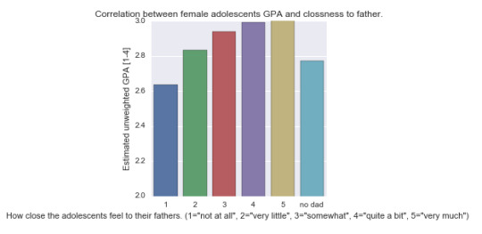
The female population: below is the bar chart of the correlation between level of closeness to adolescents’ fathers and the estimated unweight GPA for girls:

And the ANOVA and post hoc analyses:

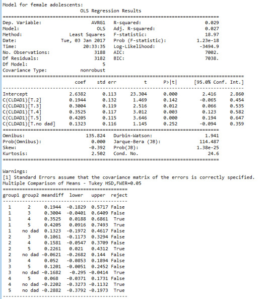
Analysis of findings:

Upon investigation of the results we see that there is a strong and significant correlation between the reported level of closeness and estimated GPA among both boys (F=18.97, p<0.0001) and girls (F=18.97, p<0.0001).

The bar charts indicate different mean values of GPA for boys and girls.

For both girls and boys, those that indicated closeness levels 3,4, and 5 (“somewhat”, “quite a bit”, and “very much”) had consistently better GPA than those who reported that they had “no dad”. Also, among both boys and girls, those that reported level 2 of closeness had significantly lower mean GPA than those that reported level 5.

The difference between boys and girls is that among girls, those that reported a level 1 closeness (“not at all”) had lower GPA comparing to those that reported levels 4 or 5 (“quite a bit” or “very much”). While among boys, those that reported a level 2 closeness (“very little”) had lower GPA than those that indicated level 4 (“quite a bit”) or higher.

In summary, adolescent’s biological sex is a moderator for the association between the unweighted GPA and level of closeness of the adolescents to their fathers.

My current Python Code:

# -*- coding: utf-8 -*- """ Created on Fri Dec 23 22:18:49 2016

@author: Farshad """

#load the packages import pandas import numpy import seaborn import matplotlib.pyplot as plt import statsmodels.formula.api as smf import statsmodels.stats.multicomp as multi #call data data=pandas.read_csv('addhealth_pds.csv',low_memory=False) # set pandas to show all columns and rows in dataframe pandas.set_option('display.max_columns',None) pandas.set_option('display.max_rows',None)

print(len(data)) # number of individuals print(len(data.columns)) # number of variables

#upper-case all the DataFrame column names data.columns=map(str.upper, data.columns)

#bug fix for display formats to avoid run time errors pandas.set_option('display.float_format', lambda x: '%f' %x)

#covert values to numerics... This avoids issues with ordering of values data["H1ED5"]=pandas.to_numeric(data["H1ED5"], errors='coerce') data["H1ED11"]=pandas.to_numeric(data["H1ED11"], errors='coerce') data["H1ED12"]=pandas.to_numeric(data["H1ED12"], errors='coerce') data["H1ED13"]=pandas.to_numeric(data["H1ED13"], errors='coerce') data["H1ED14"]=pandas.to_numeric(data["H1ED14"], errors='coerce') data["H1WP13"]=pandas.to_numeric(data["H1WP13"], errors='coerce') data["H1ED14"]=pandas.to_numeric(data["H1ED14"], errors='coerce') data["BIO_SEX"]=pandas.to_numeric(data["BIO_SEX"], errors='coerce')

#data["H1ED7"]=data["H1ED7"].astype(numpy.int64) #calculate and print count values. drpna displays the values that are missing using NaN.

#substitute NaN for values that are not significant for analysis data["BIO_SEX"]=data["BIO_SEX"].replace(6,numpy.nan) data["H1ED5"]=data["H1ED5"].replace([6,8],numpy.nan) data["H1ED5"]=data["H1ED5"].astype('category')

print('Counts for BIO_SEX') print(data['BIO_SEX'].value_counts(sort=False, dropna=False))

recode2={1:1, 2:2, 3:3, 4:4, 5:5, 6: numpy.nan, 7: 7, 8: numpy.nan} #7: non dad data['CLDAD1']=data["H1WP13"].map(recode2)

#rename categories data["CLDAD1"]=data["CLDAD1"].astype('category') data["CLDAD1"]=data["CLDAD1"].cat.rename_categories(["1","2","3","4","5","no dad",]) #bivariate graph c->Q plt.figure() g=seaborn.factorplot(x='CLDAD1',y='AVRG1', data=data, kind="bar", ci=None) g.set(ylim=(2, 3)) plt.xlabel('How close the adolescents feel to their fathers. (1="not at all", 2="very little", 3="somewhat", 4="quite a bit", 5="very much") ') plt.ylabel('Estimated unweighted GPA [1-4]') plt.title('Correlation between adolescents GPA and clossness to father.') sub1=data[['AVRG1','CLDAD1','BIO_SEX']].dropna() sub2=sub1[(sub1['BIO_SEX']==1)] #male only sub3=sub1[(sub1['BIO_SEX']==2)] #female only

g=seaborn.factorplot(x='CLDAD1',y='AVRG1', data=sub2, kind="bar", ci=None) g.set(ylim=(2, 3)) plt.xlabel('How close the adolescents feel to their fathers. (1="not at all", 2="very little", 3="somewhat", 4="quite a bit", 5="very much") ') plt.ylabel('Estimated unweighted GPA [1-4]') plt.title('Correlation between male adolescents GPA and clossness to father.')

g=seaborn.factorplot(x='CLDAD1',y='AVRG1', data=sub3, kind="bar", ci=None) g.set(ylim=(2, 3)) plt.xlabel('How close the adolescents feel to their fathers. (1="not at all", 2="very little", 3="somewhat", 4="quite a bit", 5="very much") ') plt.ylabel('Estimated unweighted GPA [1-4]') plt.title('Correlation between female adolescents GPA and clossness to father.')

#ANOVA for the first correlation print('Model for male adolescents:') model1=smf.ols(formula='AVRG1 ~ C(CLDAD1)', data=sub2) results1=model1.fit() print(results1.summary()) #Post HOC (Tukey's Honestly Significant Difference Test) for the first correlation mc1=multi.MultiComparison(sub2['AVRG1'], sub2['CLDAD1']) res1=mc1.tukeyhsd() print(res1.summary()) #ANOVA for the first correlation print('Model for female adolescents:') model2=smf.ols(formula='AVRG1 ~ C(CLDAD1)', data=sub3) results2=model2.fit() print(results2.summary()) #Post HOC (Tukey's Honestly Significant Difference Test) for the first correlation mc2=multi.MultiComparison(sub3['AVRG1'], sub3['CLDAD1']) res2=mc2.tukeyhsd() print(res2.summary())

0 notes

fanalyst · 7 years

Text

Using the Pearson Correlation:

This post is going to be a bit off-topic from my original research question. Here, I’m going to ask a new question which helps me practice using Pearson correlation. The question is:

Is there a correlation between obesity and GPA among adolescents?

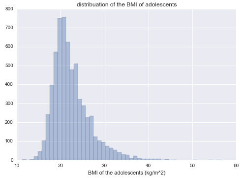
To address this question, I use the Body Mass Index as a measure for obesity. BMI is defined as:

BMI=Weight(kg)/[Height(m)]^2

World Health Organization has set forth the standards for classifying obesity in terms of the values of BMI. So I make a new variable, BMI, using my data given for weight and height. The necessary data management decisions are carried out to put the variable in shape! The following plot shows the distribution of BMI among adolescents.

For a measure of GPA, I use the AVRG1 variable that I made using the grades from 4 courses (as discussed in my previous courses). Now we can take a look at GPA versus BMI:

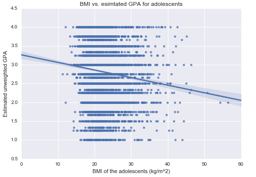
As you can see, the scatter plot does not seem very informative (I believe it would make more sense to look at BMI in a categorical way as I will discuss later); nonetheless, I will carry out the test of independence using Pearson correlation. Here’s the output of my Python code:

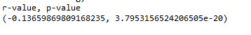
Analysis: As you can see we a small negative r-value and the p-value is very small. So the finding is significant, but the correlation is weak. The negative coefficient indicates a negative direction for linear relationship. This means that GPA decreases with increasing values of BMI. The r-square value is 0.019. This means that less than 2% of the variability in GPA can be explained using the variability in BMI. Again, the association is very weak (even though it is statistically significant)!

Note: I believe the right way to look at this problem is to categorize BMI (according to the levels suggested by WHO). This gives:

This graph is more illuminative than the one presented before; however, this is not really the topic of our interest so we leave at this!

The Python code used for this post:

# -*- coding: utf-8 -*- """ Created on Fri Dec 23 22:18:49 2016@author: Farshad """#load the packages import pandas import numpy import seaborn import matplotlib.pyplot as plt import statsmodels.formula.api as smf import statsmodels.stats.multicomp as multi import scipy.stats import itertools #call data data=pandas.read_csv('addhealth_pds.csv',low_memory=False) # set pandas to show all columns and rows in dataframe pandas.set_option('display.max_columns',None) pandas.set_option('display.max_rows',None)print(len(data)) # number of individuals print(len(data.columns)) # number of variables#upper-case all the DataFrame column names data.columns=map(str.upper, data.columns)#bug fix for display formats to avoid run time errors pandas.set_option('display.float_format', lambda x: '%f' %x)#covert values to numerics... This avoids issues with ordering of values data["H1ED5"]=pandas.to_numeric(data["H1ED5"], errors='coerce') data["H1ED11"]=pandas.to_numeric(data["H1ED11"], errors='coerce') data["H1ED12"]=pandas.to_numeric(data["H1ED12"], errors='coerce') data["H1ED13"]=pandas.to_numeric(data["H1ED13"], errors='coerce') data["H1ED14"]=pandas.to_numeric(data["H1ED14"], errors='coerce') data["H1GH60"]=pandas.to_numeric(data["H1GH60"], errors='coerce') data["H1GH59A"]=pandas.to_numeric(data["H1GH59A"], errors='coerce') data["H1GH59B"]=pandas.to_numeric(data["H1GH59B"], errors='coerce') data["AGE"]=pandas.to_numeric(data["AGE"], errors='coerce')#data["H1ED7"]=data["H1ED7"].astype(numpy.int64) #calculate and print count values. drpna displays the values that are missing using NaN. data["H1GH60"]=data["H1GH60"].replace([996,998,999],numpy.nan) data["H1GH59A"]=data["H1GH59A"].replace([96,98],numpy.nan) data["H1GH59B"]=data["H1GH59B"].replace([96,98,99],numpy.nan) data["BMI"]=data["H1GH60"]*0.453592/((data["H1GH59A"]*12+data["H1GH59B"])*0.0254)**2 data["BMIG"]=pandas.cut(data.BMI,[10,18.5,25,30,35,40,60],labels=["1", "2", "3", "4", "5", "6" ])c1=data["BMIG"].value_counts(sort=False, dropna=False) print(c1) print('Summary statistics of BMI: The body mass index of the adolescents (kg/m^2).') desc1=data["BMI"].describe() print(desc1)recode1={1:4, 2:3, 3:2, 4:1, 5:99, 96:numpy.nan, 97:99, 98:numpy.nan} # dummy 99 is when the student didn't take the course or had legitimate skip data['MATH1']=data["H1ED12"].map(recode1) data['ENGL1']=data["H1ED11"].map(recode1) data['SCIE1']=data["H1ED14"].map(recode1) data['HIST1']=data["H1ED13"].map(recode1) def AVRG1 (row): if numpy.isnan(row['MATH1']) or numpy.isnan(row['ENGL1']) or numpy.isnan(row['SCIE1']) or numpy.isnan(row['HIST1']): return numpy.nan else: i=(row['MATH1']==99)+(row['ENGL1']==99)+(row['SCIE1']==99)+(row['HIST1']==99) if i==4: return numpy.nan else: return ((row['MATH1']!=99)*row['MATH1']+(row['ENGL1']!=99)*row['ENGL1']+(row['SCIE1']!=99)*row['SCIE1']+(row['HIST1']!=99)*row['HIST1'])/(4-i) data['AVRG1']=data.apply(lambda row: AVRG1(row),axis=1)data['AVRG%']=pandas.qcut(data.AVRG1, 5, labels=["bottom20%", "bottom40%", "middle20%", "top40%", "top20%"])seaborn.distplot(data['BMI'].dropna(),kde=False) plt.xlabel('BMI of the adolescents (kg/m^2)') plt.title('distribuation of the BMI of adolescents')plt.figure() seaborn.regplot(x="BMI",y="AVRG1", fit_reg=True, data=data) plt.xlabel('BMI of the adolescents (kg/m^2)') plt.ylabel('Estimated unweighted GPA') plt.title('BMI vs. esimtated GPA for adolescents')plt.figure() seaborn.factorplot(x="BMIG",y="AVRG1", data=data, kind="bar", ci=None) plt.xlabel('BMI groups of the adolescents according to WHO. 1="underweight", 2="normal weight", 3="overweight", 4="class I obisity", 5="class II obisity", 6="class III obisity"') plt.ylabel('Estimated unweighted GPA') plt.title('BMI classes vs. esimtated GPA for adolescents') data_clean=data.dropna() print('r-value, p-value') print(scipy.stats.pearsonr(data_clean['BMI'],data_clean['AVRG1']))

0 notes

fanalyst · 7 years

Text

X-square test

In a previous post, I presented a bar chart that showed the correlation between the closeness of adolescent students to their father and the likelihood of them having to repeat a grade (please review my last 2 posts to get a better understanding of how the variables are defined and managed).

As you can see the ratio of adolescents that had to repeat a grade seemed to be increasing with decreasing closeness to their fathers for the most part. But the significance of this finding need to be investigated from statistical point of view. Since we are dealing with a categorical explanatory variable (CLDAD1) and a categorical response value (H1ED5), we use the X-square test of significance. I define my null and alternative hypotheses as follows:

H_0 = the proportion of having repeated and not having repeated a grade are equal for all the closeness levels.

H_0 = the proportion of having repeated and not having repeated a grade are NOT equal for all the closeness levels.

Below is the output of my Python code:

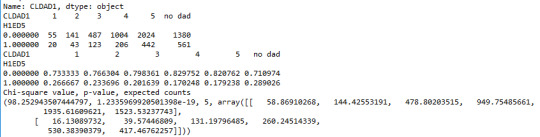
If have X^2=98.25 and p=1.2e-19, so we can reject the null and accept the alternative hypothesis. There is a strong correlation and the finding is significant, but the X-square does not provide insight as of which categories of closeness to the father are different from the others. In order to answer that question, we need to perform a post hoc analysis. Here we do additional X-square tests between every possible combination of pairs of categories of CLDAD1. There are 15 nontrivial combinations. Note that we use the Ben ferroni adjustment of p-values. So significance can be inferred for values of p that are smaller than 0.05/6=0.008. I set up a Python code to go through every possible combination of pairs of categories. Here’s the output:

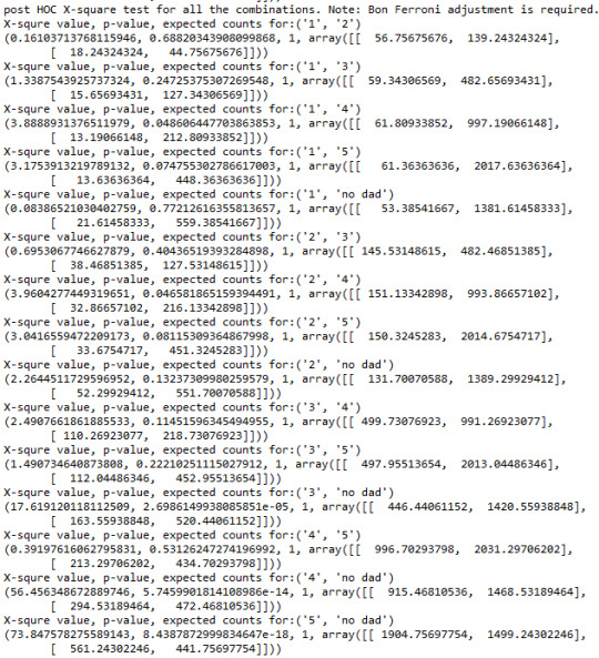
As indicated from the X-square and p values the association is strong and significant only for 3 pairs of levels of closeness. There is a significant association between the likelihood of having to repeat a grade at school for adolescents that reported they had “no dad” and those that reported closeness levels of either “somewhat”, “quite a bit” or “very much”. Those without fathers had a higher chance of repeating a grade than those that had fathers and where somewhat close, quite a bit close, or very much close to their fathers!

Short summary:

A Chi square test of independence revealed that among adolescents, the likelihood of repeating a grade at school and the level of closeness to the fathers were significantly associated, X^2=98.25, 5 df, p<0.0001.

Post hoc comparisons of rates of numbers of adolescents who had to repeat a grade by pairs of levels of closeness to their fathers revealed that students did not have fathers were more likely to repeat a grade comparing to those with fathers who indicated their closeness to their father to be average or higher. The likelihood of repeating a grade was statistically similar among all other levels of closeness.

My current Python code:

# -*- coding: utf-8 -*- """ Created on Fri Dec 23 22:18:49 2016

@author: Farshad """

#load the packages import pandas import numpy import seaborn import matplotlib.pyplot as plt import statsmodels.formula.api as smf import statsmodels.stats.multicomp as multi import scipy.stats import itertools #call data data=pandas.read_csv('addhealth_pds.csv',low_memory=False) # set pandas to show all columns and rows in dataframe pandas.set_option('display.max_columns',None) pandas.set_option('display.max_rows',None)

print(len(data)) # number of individuals print(len(data.columns)) # number of variables

#upper-case all the DataFrame column names data.columns=map(str.upper, data.columns)

#bug fix for display formats to avoid run time errors pandas.set_option('display.float_format', lambda x: '%f' %x)

#data["H1ED7"]=data["H1ED7"].astype(numpy.int64) #calculate and print count values. drpna displays the values that are missing using NaN.

#substitute NaN for values that are not significant for analysis data["H1ED5"]=data["H1ED5"].replace([6,8],numpy.nan) data["H1ED5"]=data["H1ED5"].astype('category') print('Summary statistics of H1ED5: Repeated a grade or held back a grade. {0=no, 1=yes}') desc1=data["H1ED5"].describe() print(desc1)

data['AVRG%']=pandas.qcut(data.AVRG1, 5, labels=["bottom20%", "bottom40%", "middle20%", "top40%", "top20%"])

recode2={1:1, 2:2, 3:3, 4:4, 5:5, 6: numpy.nan, 7: 7, 8: numpy.nan} #7: non dad data['CLDAD1']=data["H1WP13"].map(recode2)

#rename categories data["CLDAD1"]=data["CLDAD1"].astype('category') data["CLDAD1"]=data["CLDAD1"].cat.rename_categories(["1","2","3","4","5","no dad",]) print('Summary statistics of CLDAD1: How clsoe the adolescents feel to their fathers on scale from 1 to 5.') desc3=data['CLDAD1'].describe() print(desc3)

#bivariate bar chart data["H1ED5"]=data["H1ED5"].astype(numpy.float64) plt.figure() seaborn.factorplot(x='CLDAD1',y='H1ED5', data=data, kind="bar", ci=None) plt.xlabel('How close the adolescents feel to their fathers. (1="not at all", 2="very little", 3="somewhat", 4="quite a bit", 5="very much") ') plt.ylabel('likelihood of having to repeat a grade') plt.title('Correlation between adolescents likelihood of repeating a grade and clossness to father.') sub1=data[['AVRG1','CLDAD1']].dropna()

#X-square for the second correlation ct1=pandas.crosstab(data["H1ED5"],data["CLDAD1"]) print(ct1) colsum=ct1.sum(axis=0) colpct=ct1/colsum print(colpct) print('Chi-square value, p-value, expected counts') cs1=scipy.stats.chi2_contingency(ct1) print(cs1) #post HOC X-2 test for all combinations (Bon ferroni Adjustment requried) print('post HOC X-square test for all the combinations. Note: Bon Ferroni adjustment is required.') for pair in itertools.combinations(["1","2","3","4","5","no dad"],2): recode={pair[0]:pair[0], pair[1]:pair[1]} data['CLDAD2']=data['CLDAD1'].map(recode) ct=pandas.crosstab(data["H1ED5"],data["CLDAD2"]) print("X-squre value, p-value, expected counts for:{}".format(pair)) print(scipy.stats.chi2_contingency(ct))

0 notes

fanalyst · 7 years

Text

Is there a correlation between how close the adolescents feel to their fathers and their GPA?!

In my previous post I presented some data that indicated that the closer the adolescent students felt to their fathers, the higher GPA they had (see previous posts for more information about the how the variables are defined and managed). But is this finding statistically significant? To answer this question, we need to test the hypothesis. Since we’re dealing with a categorical explanatory variable and a quantitative response variable, we need to perform an Analysis of Variances (ANOVA). I define my null and alternative hypotheses as follows:

H_0: the mean value of estimated unweighted GPA (variable AVRG1) is the same across all categories of the variable that correspond to the closeness of the adolescents to their fathers (CLDAD1).

H_a: the mean value of estimated unweighted GPA (variable AVRG1) is NOT the same across all categories of the variable that correspond to the closeness of the adolescents to their fathers (CLDAD1).

Below is the result the output of my Python code for the ANOVA:

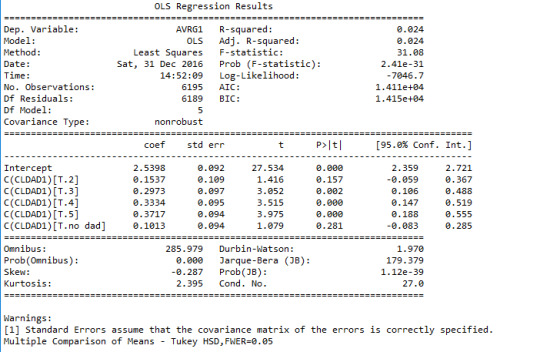
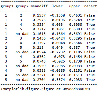
As you can see, we have a p-value of 2.41e-31<0.05. Hence the finding is significant. This means that we can safely reget the null hypothesis and accept the alternative hypothesis. But we don’t know which mean values corresponding to different categories are different a priori. We need to perfome a post HOC analysis to answer that question. Here, I use Tukey’s Honstly Significant Difference test. Here’s the output from my Python code for that:

We can interpret these outcomes a long with the bar graph that we found last time:

As you can see those adolescent without father and those who were “not close at all” to their fathers had lower GPAs comparing to those who had fathers and indicated that they are “somewhat close”, “quite a bit close”, and “very close” to their fathers.

Also those adolescents that reported “very little” and “somewhat” closeness to their fathers had less GPAs than those that reported “quite a bit” and “very much” closeness levels.

Summary of Analysis:

ANOVA revealed that the estimated unweighted GPA of adolescent students (quantitative response value) and the level of closeness to their fathers (categorical explanatory variable) were significantly dependent, F(5, 6189)= 31.08, p<0.0001.

Post HOC comparision of mean values of GPA for pairs of closeness level catagories (1=”not at all”, 2=”very little”, 3=”somewhat”, 4=”quite a bit”, 5=”very much”, “no dad”) revealed those adolescent students that did not have fathers (“no dad”) or those and those who had fathers and reported closeness level of 1 (“not at all”) to their fathers, exhibited lower mean values of GPA comparing to those that reproted closeness levels of 3 or higher (”somewhat”, ”quite a bit”, and ”very much”). Also, those student adolescents that reported closness levels of 4 or 5 (“quite a bit” or “very much”) exhibited higher mean values of GPA comparing to those that reproted closeness levels of 2 or 3 (“very little” or “some what”). All other comparisions were statistically similar.

My Current Python Code:

# -*- coding: utf-8 -*- """ Created on Fri Dec 23 22:18:49 2016

@author: Farshad """

#load the packages import pandas import numpy import seaborn import matplotlib.pyplot as plt import statsmodels.formula.api as smf import statsmodels.stats.multicomp as multi #call data data=pandas.read_csv('addhealth_pds.csv',low_memory=False) # set pandas to show all columns and rows in dataframe pandas.set_option('display.max_columns',None) pandas.set_option('display.max_rows',None)

print(len(data)) # number of individuals print(len(data.columns)) # number of variables

#upper-case all the DataFrame column names data.columns=map(str.upper, data.columns)

#bug fix for display formats to avoid run time errors pandas.set_option('display.float_format', lambda x: '%f' %x)

#data["H1ED7"]=data["H1ED7"].astype(numpy.int64) #calculate and print count values. drpna displays the values that are missing using NaN.

#substitute NaN for values that are not significant for analysis data["H1ED5"]=data["H1ED5"].replace([6,8],numpy.nan) data["H1ED5"]=data["H1ED5"].astype('category')

recode2={1:1, 2:2, 3:3, 4:4, 5:5, 6: numpy.nan, 7: 7, 8: numpy.nan} #7: non dad data['CLDAD1']=data["H1WP13"].map(recode2)

#ANOVA for the first correlation model1=smf.ols(formula='AVRG1 ~ C(CLDAD1)', data=sub1) results1=model1.fit() print(results1.summary()) #Post HOC (Tukey's Honestly Significant Difference Test) for the first correlation mc1=multi.MultiComparison(sub1['AVRG1'], sub1['CLDAD1']) res1=mc1.tukeyhsd() print(res1.summary())

0 notes

fanalyst · 7 years

Text

Visual representation of some of the managed data!

Here I resent some of the variables graphically…

Variable H1ED5: This is a categorical variable that shows whether the adolescents had to repeat any grade or were held back from a grade.

Summary statistics of H1ED5: Repeated a grade or held back a grade. {0=no, 1=yes} count 6490.000000 unique 2.000000 top 0.000000 freq 5093.000000

univariate graph:

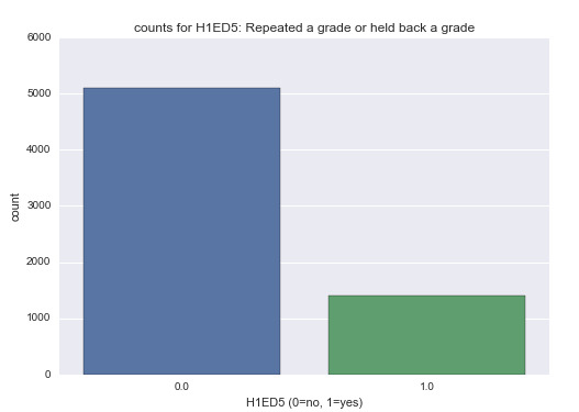
Analysis: As indicated by the bar graph, the majority of the students did not repeat any grades.

Variable AVRG1: This is a quantitative variable that provides an estimation for unweighted GPA. Summary statistics of AVRG1: approximate unweighted GPA (1-4). count 6199.000000 mean 2.808181 std 0.764065 min 1.000000 max 4.000000

univariate graph:

Analysis: The histogram shows that majority of the students had a GPA of 3 (mode).

Variable CLDAD1: A categorical variable that shows how close the adolescents feel to their fathers on a scale from 1 to 5. Summary statistics of CLDAD1: How close the adolescents feel to their fathers on scale from 1 to 5. count 6499 unique 6 top 5 freq 2467

univariate graph:

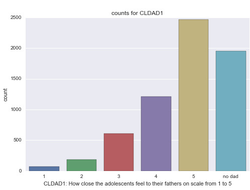
Analysis: We can see from this bar graph that most of the adolescents indicated that they are “very close” to their fathers. While a good proportion of them did not have a father.

I’m interested in knowing if there is an association between how close the adolescents feel to their father and their academic performance.

First, let’s look at the bivariate graph of CLDAD1 and AVRG1:

Analysis: The graph shows that the closer the adolescents feel to their fathers the higher their GPA are! Those students that did not have a father, exhibited low GPAs, but not as low as those that indicated “not at all” as the response to how close they are to their father.

Secondly, we look at the bivariate graph of CLDAD1 and H1ED5:

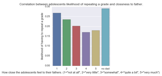
Analysis: As you can see those students that did not have a father were more likely to have to repeat a grade. Also, in general, the closer the students felt to their fathers, the lower the chance of them having to repeat a grade! This trend is valid except for those that indicated response “quite a bit” and “very much”. It turns out that those adolescents that indicated “very much,” had higher chance of repeating a grade than those that indicated “quite a bit.”

Note: The correlation between the variable mentioned above cannot be inferred unless they are statistically tested and proven to be meaningful. I am hoping to get to that in my next post.

Here’s my current Python code:

# -*- coding: utf-8 -*- """ Created on Fri Dec 23 22:18:49 2016

@author: Farshad """

#load the packages import pandas import numpy import seaborn import matplotlib.pyplot as plt #call data data=pandas.read_csv('addhealth_pds.csv',low_memory=False) # set pandas to show all columns and rows in dataframe pandas.set_option('display.max_columns',None) pandas.set_option('display.max_rows',None)

print(len(data)) # number of individuals print(len(data.columns)) # number of variables

#upper-case all the DataFrame column names data.columns=map(str.upper, data.columns)

#bug fix for display formats to avoid run time errors pandas.set_option('display.float_format', lambda x: '%f' %x)

#data["H1ED7"]=data["H1ED7"].astype(numpy.int64) #calculate and print count values. drpna displays the values that are missing using NaN.

seaborn.countplot(x='H1ED5', data=data) plt.xlabel('H1ED5 (0=no, 1=yes)') plt.title('counts for H1ED5: Repeated a grade or held back a grade')

data['AVRG%']=pandas.qcut(data.AVRG1, 5, labels=["bottom20%", "bottom40%", "middle20%", "top40%", "top20%"])

recode2={1:1, 2:2, 3:3, 4:4, 5:5, 6: numpy.nan, 7: 7, 8: numpy.nan} #7: non dad data['CLDAD1']=data["H1WP13"].map(recode2)

print('percentage of CLDAD1: (MANAGED) How close they feel to their fathers on scale from 1 to 5 (1 being not close at all and 5 being very close). 7=no Dad') p11=data["CLDAD1"].value_counts(sort=False, normalize=True, dropna=False)*100 print(p11.sort_index()) #rename categories data["CLDAD1"]=data["CLDAD1"].astype('category') data["CLDAD1"]=data["CLDAD1"].cat.rename_categories(["1","2","3","4","5","no dad",]) print('Summary statistics of CLDAD1: How clsoe the adolescents feel to their fathers on scale from 1 to 5.') desc3=data['CLDAD1'].describe() print(desc3) #univariate graph plt.figure() seaborn.countplot(x="CLDAD1",data=data) plt.xlabel('CLDAD1: How close the adolescents feel to their fathers on scale from 1 to 5') plt.title('counts for CLDAD1') #bivariate graph c->Q plt.figure() g=seaborn.factorplot(x='CLDAD1',y='AVRG1', data=data, kind="bar", ci=None) g.set(ylim=(2, 3)) plt.xlabel('How close the adolescents feel to their fathers. (1="not at all", 2="very little", 3="somewhat", 4="quite a bit", 5="very much") ') plt.ylabel('Estimated unweighted GPA [1-4]') plt.title('Correlation between adolescents GPA and clossness to father.') #bivariate bar chart data["H1ED5"]=data["H1ED5"].astype(numpy.float64) plt.figure() seaborn.factorplot(x='CLDAD1',y='H1ED5', data=data, kind="bar", ci=None) plt.xlabel('How close the adolescents feel to their fathers. (1="not at all", 2="very little", 3="somewhat", 4="quite a bit", 5="very much") ') plt.ylabel('likelihood of having to repeat a grade') plt.title('Correlation between adolescents likelihood of repeating a grade and clossness to father.')

0 notes

fanalyst · 7 years

Text

Some Data Management Decisions!

In order to work with my data, I need to process some of the data to make them more sensible. My Python code includes data management decisions corresponding to several variables, but here I’m going to discuss the main ones. (For explanation of the objective of the analysis and more information about parameters involved, please see the previous two posts.)

Variables H1ED5 & H1ED7: did you ever skipped a grade? & Have you ever received an out-of-school suspension from school?

-Possible responses:

0 no

1 yes

6 refuse

8 I don’t know

-Data management decisions for these variables:

Here we code out the missing data since the dummy indices 6 and 8 do not convey useful information for our analysis so I substitute them with “nan”s.

Variables H1ED12, H1ED11, H1ED14, and H1ED13: What was your grade in mathematics/English/science/history?

Possible responses:

1 A

2 B

3 C

4 D

5 didn’t take this subject

96 refuse

97 legitimate skip

98 don’t know

-Data management decisions for these variables:

Firstly, we note that the numeral values corresponding to letter grades are counter-intuitive (at least to me)! So I relabeled these variable such that 4--> A, 3-->B, 2-->C, 1--> D. I code out dummy indices 96 and 98 to “nan”s. categories 5, and 97 convey useful information so they should be coded as valid data. So I map them as such: 96 --> 99, 98 --> 99 where the newly-defined dummy 99 represent some type of legitimate skip. I call the managed variables MATH1, ENGL1, SCIE1, and HIST1 respectively.

New variable AVRG1: estimated unweighted-GPA based on the scores from MATH1, ENGL1, SCIE1, and HIST1.

-Possible responses:

Continuous numeric values [1-4] and “nan” when the GPA cannot be defined because of missing data.

-Data management decisions for these variables:

I am interested in making an aggregate variable from the grades in the aforementioned courses. So I defined an estimated GPA based on the grades from these courses. This can be done by finding the mean of these 4 variables for all the observations. There are two important caveats here: 1- If the there are any missing data for the 4 variables (nan values), the AVRG1 should obtain the value “nan”. 2- If there are legitimate skips (category 99) for any of the 4 variables, the AVRG1 should be calculated from the rest of the variables that have valid values (1-4). I coded this by using nested conditional statements in Python. (I’m sure there is a more efficient way to do it. I’m newbie with Python so if you know how, please let me know!)

New variable AVRG%: quintile distribution values corresponding to AVRG1.

-Possible responses:

top20% students with GPA at the top 20% of the population

top40% students with GPA at the top 40% of the population

middle20% students with GPA at the middle 20% of the population

bottom40% students with GPA at the bottom 40% of the population

bottom20% students with GPA at the bottom 20% of the population

nan when the GPA cannot be calculated (due to missing data, etc.)

-Data management decisions for this variable:

Since I want to identify students with low or high academic performance, it makes sense to define a new categorical value based on quintiles. So I collapse categories in AVRG1 to get percentiles as defined above.

Frequency distributions (output from Python):

counts for H1ED5: Repeated a grade or held back a grade. {0=no, 1=yes, nan=missing}

0.000000 5093

1.000000 1397

nan 14

Name: H1ED5, dtype: int64

percentage of H1ED5: Repeated a grade or held back a grade. {0=no, 1=yes, nan=missing}

0.000000 78.305658

1.000000 21.479090

nan 0.215252

Name: H1ED5, dtype: float64

counts for H1ED7: Out-of-school suspension. {0=no, 1=yes, nan=missing}

0.000000 4687

1.000000 1801

nan 16

Name: H1ED7, dtype: int64

percentage of H1ED7: Out-of-school suspension. {0=no, 1=yes, nan=missing}

0.000000 72.063346

1.000000 27.690652

nan 0.246002

***NOTE: The following values are evaluated after eliminating observations that where not in the bottom 20 percentile of the population.***

count of CLDAD1: (MANAGED) How close they feel to their fathers on scale from 1 to 5 (1 being not close at all and 5 being very close). 7=no Dad

1.000000 21

2.000000 42

3.000000 109

4.000000 213

5.000000 384

7.000000 489

nan 1

Name: CLDAD1, dtype: int64

percentage of CLDAD1: (MANAGED) How close they feel to their fathers on scale from 1 to 5 (1 being not close at all and 5 being very close). 7=no Dad

1.000000 1.667990

2.000000 3.335981

3.000000 8.657665

4.000000 16.918189

5.000000 30.500397

7.000000 38.840349

nan 0.079428

Name: CLDAD1, dtype: float64

The frequency table for H1ED5 shows that 21.48% of the students had to repeat at least one grade. After data management, now we have 0.21% of data that are missing.

Similarly, for H1ED7, about 0.25% of the data are missing.

After limiting our population to those with GPAs in the bottom 20% of the total population, the frequency table of the managed data (CLDAD1) is derived. Comparing these values to the values of the total population (see last post), we see that students with low GPA indicate lower levels of closeness to their father. Also there are more students without fathers in this group. There is only one missing datum for this category.

My current Python code:

# -*- coding: utf-8 -*-

"""

Created on Fri Dec 23 22:18:49 2016

@author: Farshad

"""

#load the packages

import pandas

import numpy

#call data

data=pandas.read_csv('addhealth_pds.csv',low_memory=False)

print(len(data)) # number of individuals

print(len(data.columns)) # number of variables

#upper-case all the DataFrame column names

data.columns=map(str.upper, data.columns)

#bug fix for display formats to avoid run time errors

pandas.set_option('display.float_format', lambda x: '%f' %x)

#covert values to numerics... This avoids issues with ordering of values

data["H1ED5"]=data["H1ED5"].convert_objects(convert_numeric=True)

data["H1ED7"]=data["H1ED7"].convert_objects(convert_numeric=True)

data["H1ED11"]=data["H1ED11"].convert_objects(convert_numeric=True)

data["H1ED12"]=data["H1ED12"].convert_objects(convert_numeric=True)

data["H1ED13"]=data["H1ED13"].convert_objects(convert_numeric=True)

data["H1ED14"]=data["H1ED14"].convert_objects(convert_numeric=True)

data["H1ED16"]=data["H1ED16"].convert_objects(convert_numeric=True)

data["H1WP8"]=data["H1WP8"].convert_objects(convert_numeric=True)

data["H1WP9"]=data["H1WP9"].convert_objects(convert_numeric=True)

data["H1WP10"]=data["H1WP10"].convert_objects(convert_numeric=True)

data["H1WP13"]=data["H1WP13"].convert_objects(convert_numeric=True)

data["H1WP14"]=data["H1WP14"].convert_objects(convert_numeric=True)

data["H1PF1"]=data["H1PF1"].convert_objects(convert_numeric=True)

#data['H1ED5'] = pandas.to_numeric(data['H1ED5'])

#calculate and print count values. drpna displays the values that are missing using NaN.

#substitute NaN for values that are not significant for analysis

data["H1ED5"]=data["H1ED5"].replace([6,8],numpy.nan)

print('counts for H1ED5: Repeated a grade or held back a grade. {0=no, 1=yes, nan=missing}')

c1=data["H1ED5"].value_counts(sort=False, dropna=False)

print(c1.sort_index())

print('percentage of H1ED5: Repeated a grade or held back a grade. {0=no, 1=yes, nan=missing}')

p1=data["H1ED5"].value_counts(sort=False, normalize=True, dropna=False)*100

print(p1.sort_index())

#substitute NaN for values that are not significant for analysis

data["H1ED7"]=data["H1ED7"].replace([6,8],numpy.nan)

print('counts for H1ED7: Out-of-school suspension. {0=no, 1=yes, nan=missing}')

c2=data["H1ED7"].value_counts(sort=False, dropna=False)

print(c2.sort_index())

print('percentage of H1ED7: Out-of-school suspension. {0=no, 1=yes, nan=missing}')

p2=data["H1ED7"].value_counts(sort=False, normalize=True, dropna=False)*100

print(p2.sort_index())

recode1={1:4, 2:3, 3:2, 4:1, 5:99, 96:numpy.nan, 97:99, 98:numpy.nan} # dummy 99 is when the student didn't take the course or had legitimate skip

data['MATH1']=data["H1ED12"].map(recode1)

data['ENGL1']=data["H1ED11"].map(recode1)

data['SCIE1']=data["H1ED14"].map(recode1)

data['HIST1']=data["H1ED13"].map(recode1)

def AVRG1 (row):

if numpy.isnan(row['MATH1']) or numpy.isnan(row['ENGL1']) or numpy.isnan(row['SCIE1']) or numpy.isnan(row['HIST1']):

return numpy.nan

else:

i=(row['MATH1']==99)+(row['ENGL1']==99)+(row['SCIE1']==99)+(row['HIST1']==99)

if i==4:

return numpy.nan

else:

return ((row['MATH1']!=99)*row['MATH1']+(row['ENGL1']!=99)*row['ENGL1']+(row['SCIE1']!=99)*row['SCIE1']+(row['HIST1']!=99)*row['HIST1'])/(4-i)

data['AVRG1']=data.apply(lambda row: AVRG1(row),axis=1)

sub3=data[['AID','MATH1','ENGL1','SCIE1','HIST1','AVRG1']]

print(sub3.head(n=25))

data['AVRG%']=pandas.qcut(data.AVRG1, 5, labels=["bottom20%", "bottom40%", "middle20%", "top40%", "top20%"])

print(pandas.crosstab(data['AVRG%'], data['AVRG1']))

print('counts for AVRG%: Quintile GPA')

p3=data["AVRG%"].value_counts(sort=False, dropna=False)

print('percentage of AVRG%: Quintile GPA')

p3=data["AVRG%"].value_counts(sort=False, normalize=True, dropna=False)*100

print(p3)

sub4=data[['AID','AVRG%','AVRG1']]

print(sub4.head(n=25))

recode2={1:1, 2:2, 3:3, 4:4, 5:5, 6: numpy.nan, 7: 7, 8: numpy.nan} #7: non dad

data['CLDAD1']=data["H1WP13"].map(recode2)

print('count of H1WP13: How close they feel to their fathers on scale from 1 to 5 (1 being not close at all and 5 being very close). 6= refuse to answer, 7=no Dad, 8= I dont know')

c11=data["H1WP13"].value_counts(sort=False, dropna=False)

print(c11.sort_index())

print('percentage of H1WP13: How close they feel to their fathers on scale from 1 to 5 (1 being not close at all and 5 being very close). 6= refuse to answer, 7=no Dad, 8= I dont know')

p11=data["H1WP13"].value_counts(sort=False, normalize=True, dropna=False)*100

print(p11.sort_index())

print('percentage of CLDAD1: (MANAGED) How close they feel to their fathers on scale from 1 to 5 (1 being not close at all and 5 being very close). 7=no Dad')

p11=data["CLDAD1"].value_counts(sort=False, normalize=True, dropna=False)*100

print(p11.sort_index())

#getting a sub-set by eliminating a number of observations

sub1=data[(data["AVRG%"]=="bottom20%")]

sub2=sub1.copy()

print('***NOTE: The following values are evaluated after eliminating observations that where not in the bottom 20 percentile of the population.***' )

print('count of CLDAD1: (MANAGED) How close they feel to their fathers on scale from 1 to 5 (1 being not close at all and 5 being very close). 7=no Dad')

c11=sub2["CLDAD1"].value_counts(sort=False, dropna=False)

print(c11.sort_index())

print('percentage of CLDAD1: (MANAGED) How close they feel to their fathers on scale from 1 to 5 (1 being not close at all and 5 being very close). 7=no Dad')

p11=sub2["CLDAD1"].value_counts(sort=False, normalize=True, dropna=False)*100

print(p11.sort_index())

0 notes

fanalyst · 7 years

Text

Starting my code in Python!

Based on the research project I defined in my previous post, I have set up a python code (using pandas package) to analyze the data. I will use this code as a platform and build up on it as I progress. For now, I want to look at the count and frequency distribution of a number of parameters.

Please scroll down to the end of this post to see the python code. Note that the code requires the “addhealth_pds.csv” to run. To illustrate how my code works, I am writing out the frequency distribution and counts for 4 of my parameters for all the 6504 observations.

a) Frequency table for how many of the students had to repeat (or were held back) a grade at school

counts for H1ED5: Repeated a grade or held back a grade. {0=no, 1=yes, 6= refuse, 8= I don’t know}

0 5093

1 1397

6 5

8 9

Name: H1ED5, dtype: int64

percentage of H1ED5: Repeated a grade or held back a grade. {0=no, 1=yes, 6= refuse, 8= I don’t know}

0 78.305658

1 21.479090

6 0.076876

8 0.138376

Name: H1ED5, dtype: float64

b) Frequency table for how many students at out-of-school suspensions.

counts for H1ED7: Out-of-school suspension. {0=no, 1=yes, 6= refuse, 8= I don’t know, nan=missing}

0.000000 4687

1.000000 1801

6.000000 5

8.000000 8

nan 3

Name: H1ED7, dtype: int64

percentage of H1ED7: Out-of-school suspension. {0=no, 1=yes, 6= refuse, 8= I don’t know, nan=missing}

0.000000 72.063346

1.000000 27.690652

6.000000 0.076876

8.000000 0.123001

nan 0.046125

Name: H1ED7, dtype: float64

c) Frequency table for the students’ grades in mathematics

count for H1ED12: Grade in mathematics {1=A, 2=B, 3=C, 4=D, 5=didn’t take this subject, 96=refuse, 97= legitimate skip, 98= I don’t know}

1 1552

2 1899

3 1521

4 950

5 353

6 69

96 4

97 128

98 28

Name: H1ED12, dtype: int64

percentage of H1ED12: Grade in mathematics {1=A, 2=B, 3=C, 4=D, 5=didn’t take this subject, 96=refuse, 97= legitimate skip, 98= I don’t know}

1 23.862239

2 29.197417

3 23.385609

4 14.606396

5 5.427429

6 1.060886

96 0.061501

97 1.968020

98 0.430504

Name: H1ED12, dtype: float64

d) Frequency table for how close the students feel to their fathers

count of H1WP13: How close they feel to their fathers on scale from 1 to 5 (1 being not close at all and 5 being very close). 6= refuse to answer, 7=no Dad, 8= I don’t know

1 75

2 184

3 610

4 1211

5 2467

6 4

7 1952

8 1

Name: H1WP13, dtype: int64

percentage of H1WP13: How close they feel to their fathers on scale from 1 to 5 (1 being not close at all and 5 being very close). 6= refuse to answer, 7=no Dad, 8= I don’t know

1 1.153137

2 2.829028

3 9.378844

4 18.619311

5 37.930504

6 0.061501

7 30.012300

8 0.015375

Name: H1WP13, dtype: float64

Out of curiosity, I wanted to see the last frequency distribution (d) among those students that have had to “repeat at least one grade” AND have had “out-of-school suspension”.

***NOTE: The following values are evaluated after eliminating observations that did not have both "out-of-school suspension" and "repeated or held-back grade(s)".***

count of H1WP13: How close they feel to their fathers on scale from 1 to 5 (1 being not close at all and 5 being very close). 6= refuse to answer, 7=no Dad, 8= I don’t know

1 17

2 18

3 51

4 91

5 188

6 2

7 320

Name: H1WP13, dtype: int64

percentage of H1WP13: How close they feel to their fathers on scale from 1 to 5 (1 being not close at all and 5 being very close). 6= refuse to answer, 7=no Dad, 8= I don’t know

1 2.474527

2 2.620087

3 7.423581

4 13.245997

5 27.365357

6 0.291121

7 46.579330

As you can see, in the aforementioned group of students, there a higher percentage of students that do not have a dad (46.6% comparing to 30.0%). However, in both groups, most of the students indicated “very close” relationship with their parents.

Note that in (b), “nan” corresponds to the observations for which the data are missing (in this case it comprises about 0.05% of the population).

Below is my current python code:

# -*- coding: utf-8 -*- """ Created on Fri Dec 23 22:18:49 2016

@author: Farshad """

#load the packages import pandas import numpy #call data data=pandas.read_csv('addhealth_pds.csv',low_memory=False)

print(len(data)) # number of individuals print(len(data.columns)) # number of variables

#upper-case all the DataFrame column names data.columns=map(str.upper, data.columns)

#bug fix for display formats to avoid run time errors pandas.set_option('display.float_format', lambda x: '%f' %x)

#covert values to numerics... This avoids issues with ordering of values

data["H1ED5"]=data["H1ED5"].convert_objects(convert_numeric=True) data["H1ED7"]=data["H1ED7"].convert_objects(convert_numeric=True) data["H1ED11"]=data["H1ED11"].convert_objects(convert_numeric=True) data["H1ED12"]=data["H1ED12"].convert_objects(convert_numeric=True) data["H1ED13"]=data["H1ED13"].convert_objects(convert_numeric=True) data["H1ED14"]=data["H1ED14"].convert_objects(convert_numeric=True) data["H1ED16"]=data["H1ED16"].convert_objects(convert_numeric=True) data["H1WP8"]=data["H1WP8"].convert_objects(convert_numeric=True) data["H1WP9"]=data["H1WP9"].convert_objects(convert_numeric=True) data["H1WP10"]=data["H1WP10"].convert_objects(convert_numeric=True) data["H1WP13"]=data["H1WP13"].convert_objects(convert_numeric=True) data["H1WP14"]=data["H1WP14"].convert_objects(convert_numeric=True) data["H1PF1"]=data["H1PF1"].convert_objects(convert_numeric=True)

#data['H1ED5'] = pandas.to_numeric(data['H1ED5'])

#calculate and print count values. drpna displays the values that are missing using NaN.

print('counts for H1ED5: Repeated a grade or held back a grade. {0=no, 1=yes, 6= refuse, 8= I dont know}') c1=data["H1ED5"].value_counts(sort=False, dropna=False) print(c1.sort_index()) print('percentage of H1ED5: Repeated a grade or held back a grade. {0=no, 1=yes, 6= refuse, 8= I dont know}') p1=data["H1ED5"].value_counts(sort=False, normalize=True, dropna=False)*100 print(p1.sort_index())

print('counts for H1ED7: Out-of-school suspension. {0=no, 1=yes, 6= refuse, 8= I dont know, nan=missing}') c2=data["H1ED7"].value_counts(sort=False, dropna=False) print(c2.sort_index()) print('percentage of H1ED7: Out-of-school suspension. {0=no, 1=yes, 6= refuse, 8= I dont know, nan=missing}') p2=data["H1ED7"].value_counts(sort=False, normalize=True, dropna=False)*100 print(p2.sort_index())

print('count for H1ED12: Grade in mathematics {1=A, 2=B, 3=C, 4=D, 5=didnt take this subject, 96=refuse, 97= legitimate skip, 98= I dont know}') c4=data["H1ED12"].value_counts(sort=False, dropna=False) print(c4.sort_index()) print('percentage of H1ED12: Grade in mathematics {1=A, 2=B, 3=C, 4=D, 5=didnt take this subject, 96=refuse, 97= legitimate skip, 98= I dont know}') p4=data["H1ED12"].value_counts(sort=False, normalize=True, dropna=False)*100 print(p4.sort_index())

print('count of H1WP13: How close they feel to their fathers on scale from 1 to 5 (1 being not close at all and 5 being very close). 6= refuse to answer, 7=no Dad, 8= I dont know') c11=data["H1WP13"].value_counts(sort=False, dropna=False) print(c11.sort_index()) print('percentage of H1WP13: How close they feel to their fathers on scale from 1 to 5 (1 being not close at all and 5 being very close). 6= refuse to answer, 7=no Dad, 8= I dont know') p11=data["H1WP13"].value_counts(sort=False, normalize=True, dropna=False)*100 print(p11.sort_index())

#getting a sub-set by eliminating a number of observations sub1=data[(data["H1ED7"]==1) & (data["H1ED5"]==1)] sub2=sub1.copy()

print('***NOTE: The following values are evaluated after eliminating observations that did not have both "out-of-school suspension" and "repeated or held-back grade(s)".***' ) print('count of H1WP13: How close they feel to their fathers on scale from 1 to 5 (1 being not close at all and 5 being very close). 6= refuse to answer, 7=no Dad, 8= I dont know') c11=sub2["H1WP13"].value_counts(sort=False, dropna=False) print(c11.sort_index()) print('percentage of H1WP13: How close they feel to their fathers on scale from 1 to 5 (1 being not close at all and 5 being very close). 6= refuse to answer, 7=no Dad, 8= I dont know') p11=sub2["H1WP13"].value_counts(sort=False, normalize=True, dropna=False)*100 print(p11.sort_index())

0 notes

fanalyst · 7 years

Text

My first Data Analysis Project!

Primary research question: Is there a correlation between the quality of parent-adolescent relationship and adolescents’ performance at school?

Context (literature review): Parent-adolescent relationship has been the focus of many studies performed in the past [1-3]. In particular, many studies have investigated the effect of parenting style and academic achievements [4, 5]. For example, Dornbusch et al.[5] found out that authoritative parenting style affects the students’ grades in a positive manner, while authoritarian and permissive parenting styles have negative impacts on the students’ grades. None of the studies that I came across have examined the effect of the quality of the relationships on the academic achievements. In this project, I like to find out if there is any correlation between the quality of adolescent-parent relationship from the adolescents’ perspective and their academic performance. Are satisfactory relationships with parents related to better grades at school?

As a secondary topic, I would like to know if the quality of parent-adolescent relationship is associated with success in mathematics. Researchers have investigated the relationship between parental involvement and mathematical achievements [6, 7], but the quality of such relationships has not been the focus of these studies. In this project, I am going to investigate the existence of a correlation between mathematical achievement and the quality of adolescent-parent relationship from the students’ perspective.

Hypothesis: Better academic performance of the adolescents is associated with better quality of parent-adolescent relationships.

Secondary research question: Is mathematical achievement associated with the quality of adolescent-parent relationship from the students’ perspective?

Selected dataset: This project will be conducted based on the data gathered in the National Longitudinal Study of Adolescent Health (AddHealth). AddHealth is a school-based survey of adolescents in grades 7-12 in the United States.

AddHealth consists of 40 sections, each of which correspond to a particular aspect of the longitudinal study. For the purpose of this project, I limit my investigation to sections 5 (Academics and Education), 16 (Relations with parents), and 18 (Personality and Family).

Search terms used: parent-adolescent relationship, academic performance, mathematical achievements

References:

[1] Farrell, Albert D., and Kamila S. White. "Peer influences and drug use among urban adolescents: Family structure and parent–adolescent relationship as protective factors." Journal of consulting and clinical psychology 66.2 (1998): 248.

[2] McGue, Matt, et al. "Perceptions of the parent-adolescent relationship: a longitudinal investigation." Developmental psychology 41.6 (2005): 971.

[3] Steinberg, Laurence. "We know some things: Parent–adolescent relationships in retrospect and prospect." Journal of research on adolescence 11.1 (2001): 1-19.

[4] Weiss, Laura H., and J. Conrad Schwarz. "The relationship between parenting types and older adolescents' personality, academic achievement, adjustment, and substance use." Child development 67.5 (1996): 2101-2114.

[5] Dornbusch, Sanford M., et al. "The relation of parenting style to adolescent school performance." Child development (1987): 1244-1257.

[6] Muller, Chandra. "Gender differences in parental involvement and adolescents' mathematics achievement." Sociology of Education (1998): 336-356.

[7] Muller, Chandra. "Maternal employment, parent involvement, and mathematics achievement among adolescents." Journal of Marriage and the Family (1995): 85-100.

1 note · View note