
Last Seen Blogs

quadrantmodelquotes
Quadrant Model Quotes from 2013 Lectures

reinellemae
GAPPI C-PHA-9

knitsbyice
Knits By Ice


kinnabarii-blog
moved.
Text
WEEK 4
This week I decided to plot the following variables:
- For uni-variate graphs, I plotted:
Crater diameter
Crater depth-to-diameter ratio
Crater latitude
Ejecta morphology
- For bi-variate graphs, I plotted:
Crater depth vs crater diameter
Crater diameter vs latitude
Crater depth-to-diameter ratio vs latitude
I also decided to get a simple statistical description of the following variables:
Crater diameter
Crater depth-to-diameter ratio
Here is the Python code I wrote for this week’s assignement:
# Import panda library
import pandas
import numpy
import seaborn
import matplotlib.pyplot as plt
# Import CSV dataset
data = pandas.read_csv('C:\\Users\\Sophie et Bruno\\Documents\\Coursera\\Data Analysis and Interpretation\\marscrater_pds.csv',low_memory=False)
#Set PANDAS to show all columns in DataFrame
pandas.set_option('display.max_columns', None)
#Set PANDAS to show all rows in DataFrame
pandas.set_option('display.max_rows', None)
# Remove unused columns from dataset
data = data.drop('CRATER_ID',1)
data = data.drop('CRATER_NAME',1)
data = data.drop('MORPHOLOGY_EJECTA_3',1)
data = data.drop('NUMBER_LAYERS',1)
# Select rows with diameter more than 3km and non-empty morphology description
sub1 = data[(data['DIAM_CIRCLE_IMAGE']>3) & (data['MORPHOLOGY_EJECTA_1']!=' ')]
#print(sub1)
# Make a copy of the subset data created on Week 2
sub2=sub1.copy()
# DATA MANAGEMENT DECISION NUMBER 1 :
# I want to keep only the rows where there is a single description
# for primary morphology (i.e. the variable MORPHOLOGY_EJECTA_1 contains no slash)
# (coding found on stackoverflow)
sub2[sub2['MORPHOLOGY_EJECTA_1'].str.contains("/")]=numpy.nan
# DATA MANAGEMENT DECISION NUMBER 2 :
# Compute the depth-to-diameter ratio as a percentage
sub2['d2D_RATIO'] = (sub2['DEPTH_RIMFLOOR_TOPOG'] / sub2['DIAM_CIRCLE_IMAGE']) * 100
sub2['d2D_RATIO']=sub2['d2D_RATIO'].replace(0, numpy.nan)
# Make a copy of the subset data created on Week 3
sub3=sub2.copy()
# Plot crater diameter as a bar graph
seaborn.distplot(sub3["DIAM_CIRCLE_IMAGE"].dropna(), kde=False, hist_kws={'log':True});
plt.xlabel('Crater diameter (km)')
plt.ylabel('Occurrences')
plt.title('Crater diameter distribution')
# Plot crater depth-to-diameter ratio as a bar graph
seaborn.distplot(sub3["d2D_RATIO"].dropna(), kde=False);
plt.xlabel('Depth-to-diameter ratio in percent')
plt.ylabel('Occurrences')
plt.title('Depth-to-diameter ratio distribution')
# Plot crater latitude as a bar graph
seaborn.distplot(sub3["LATITUDE_CIRCLE_IMAGE"].dropna(), kde=False);
plt.xlabel('Latitude (degrees)')
plt.ylabel('Occurrences')
plt.title('Crater latitude distribution')
# Plot ejecta morphology as a bar graph
seaborn.countplot(x="MORPHOLOGY_EJECTA_1", data=sub3, order = sub3['MORPHOLOGY_EJECTA_1'].value_counts().index)
plt.xlabel('Ejecta morphology')
plt.xticks(rotation=90)
plt.ylabel('Occurrences')
plt.title('Ejecta morphology distribution')
print('Describe depth-to-diameter ratio')
desc1 = sub3['d2D_RATIO'].describe()
print(desc1)
print('Describe crater diameter')
desc2 = sub3['DIAM_CIRCLE_IMAGE'].describe()
print(desc2)
print('Describe ejecta morphology')
desc3 = sub3['MORPHOLOGY_EJECTA_1'].describe()
print(desc3)
# basic scatterplot: depth vs diameter
scat1 = seaborn.regplot(x="DIAM_CIRCLE_IMAGE", y="DEPTH_RIMFLOOR_TOPOG", fit_reg=False, data=sub3)
plt.xlabel('Diameter (km)')
plt.ylabel('Depth (km)')
plt.title('Scatterplot for the Association Between depth and diameter')
# basic scatterplot: d2D vs latitude
scat1 = seaborn.regplot(x="LATITUDE_CIRCLE_IMAGE", y="DIAM_CIRCLE_IMAGE", fit_reg=False, data=sub3)
plt.xlabel('Latitude (degrees)')
plt.ylabel('Diameter (km)')
plt.title('Scatterplot for the Association Between diameter and latitude')
# basic scatterplot: d2D vs latitude
scat1 = seaborn.regplot(x="LATITUDE_CIRCLE_IMAGE", y="d2D_RATIO", fit_reg=False, data=sub3)
plt.xlabel('Latitude (degrees)')
plt.ylabel('Depth-to-diameter ratio (%)')
plt.title('Scatterplot for the Association Between depth-to-diameter ratio and latitude')
And here are the results it yielded:
Describe depth-to-diameter ratio
count 35118.000000
mean 6.496546
std 4.101684
min 0.117825
25% 2.835569
50% 6.004619
75% 9.756098
max 23.076923
Name: d2D_RATIO, dtype: float64
Describe crater diameter
count 38296.000000
mean 9.098591
std 11.696816
min 3.010000
25% 3.810000
50% 5.260000
75% 9.010000
max 263.350000
Name: DIAM_CIRCLE_IMAGE, dtype: float64
Describe ejecta morphology
count 38296
unique 28
top Rd
freq 22842
Name: MORPHOLOGY_EJECTA_1, dtype: object
As can be seen from the results above, the distribution of crater diameters is very scattered : the mean is around 9km, but the standard deviation is nearly 12km, indicating a high variability of the crater diameter, as expected.
On the other hand, the depth-to-diameter ratio seems to be much less scattered : the mean value is around 6.5%, with a standard deviation around 4%, indicating that this ratio is less “volatile” than the diameter itself.
The third statistical description shows that there are 28 different types of ejecta morphologies in our subset data, but the “Rd” morphology (radial ejecta) is by far the most common one.
Here are the uni-variate graphs generated by the program :
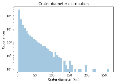
This graph is displayed with a logarithmic y-scale in order to make it more readable. As expected, it shows that the vast majority of craters have smaller diameters, while the larger craters are less frequent.
Up to about 120km, this variable (diameter) shows a consistent negative slope, which confirms the relationship mentioned earlier in the project : the larger the craters, the less frequently they occur. Above 120km size, the number of craters are too small and it makes no sense to try to derive any statistics from those.
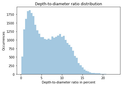
This graph shows a bi-modal distribution for the depth-to-diameter ratio. There is a first, larger peak around 2-3%, and a secondary, smaller peak aroud 10%. This might be explained by the 2 main terrains that are encountered on the surface of Mars : a hard, volcanic rock terrain and a softer, ice-rich terrain. In the soft, ice-rich terrain that are prominent at higher latitudes, the craters tend to be shallower because they get filled with the fluid-rich materials generated by the impact, whereas in the hard, volcanic terrain, there are less fluids and hence the craters don’t get filled as much after the impact.
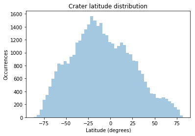
The latitude of craters shows a normal, mono-modal distribution, with a peak around -20° of latitude. It is interesting to note that above +/- 80° of latitude, there are virtually no craters accounted for. This could be a bias generated by the way the data was acquired (maybe the probe that scouted the surface of Mars didn’t fly above the poles as much as it did above lower latitudes).
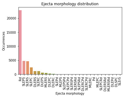
The distribution of ejecta morphology is self-explanatory and confirms that radial ejecta are by far the most common.
Here are the bi-variate graphs generated by the program :
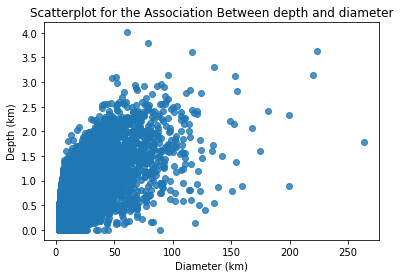
When we plot crater depth vs crater diameter, it is obvious that there is a relationship between these 2 variables : the greater the diameter, the greater the depth. Here is the same graph plotted with the best-fit linear regression :

From this graph we can see that the relationship between depth and diameter is somehow weak, as there is a high variability of the scattered plot around the best-fit linear regression.
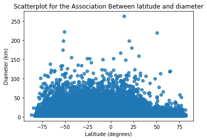
When we plot diameter vs latitude, we see that there is no relationship between these 2 variables : the location of the impact has apparently no influence on its amplitude.
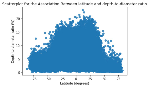
The most interesting plot in my opinion is the one above : it shows the depth-to-diameter ratio vs latitude.
From this graph it is quite obvious that this ratio is higher for lower latitudes (between -40° and +40° approximately). This correlates with the hard, volcanic terrains which are concentrated around these lower latitudes.
On the other hand, the depth-to-diameter ratio is lower for higher latitudes (below -40° and above +40°). This correlates with the soft, ice-rich terrains which are concentrated around these higher latitudes (closer to the poles).
As a conclusion, this last graph is a confirmation of the hypothesis made at the beginning of this research project : as stated earlier by previous research, the depth-to-diameter ratio depends on the type of terrain where the impact occrus. The harder the terrain, the higher the depth-to-diameter ratio, and the softer the terrain, the lower the depth-to-diameter ratio.
0 notes
Text
WEEK 3
This week I made several data management decisions, based on the frequency distributions computed last week, and also based on the fact that I wanted my data to be displayed in a more clear and more simple manner.
Here are the 4 data management decisions I made :
- Decision 1 : keep only the craters whose primary morphology is described by a single code, and ignore craters that have multiple descriptions (i.e. keep only the craters for which the MORPHOLOGY_EJECTA_1 variable does NOT contain a slash);
- Decision 2 : compute the depth-to-diameter ratio and save it as a new variable called d2D_RATIO. This value is in percents, and is computed simply as (depth/diameter)*100;
- Decision 3 : split the crater diameters into 7 ranges to make the frequency distribution easier to interpret. The ranges are 3-5km, 5-10km, 10-20km, 20-50km, 50-100km, 100-200km and 200-500km;
- Decision 4 : also split the depth-to-diameter ratio into 5 ranges for clarity. The ranges are 0-5%, 5-10%, 10-15%, 15-20% and 20-25%.
After implementing these 4 decisions on my data, I computed the frequency distributions for the following 3 variables :
- Crater diameter
- Crater depth-to-diameter ratio
- Ejecta morphology
Here is the Python code I have used for this week’s assignement :
# Import panda library
import pandas
import numpy
# Import CSV dataset
data = pandas.read_csv('marscrater_pds.csv',low_memory=False)
# Remove unused columns from dataset
data = data.drop('CRATER_ID',1)
data = data.drop('CRATER_NAME',1)
data = data.drop('MORPHOLOGY_EJECTA_3',1)
data = data.drop('NUMBER_LAYERS',1)
# Select rows with diameter more than 3km and non-empty morphology description
sub1 = data[(data['DIAM_CIRCLE_IMAGE']>3) & (data['MORPHOLOGY_EJECTA_1']!=' ')]
#print(sub1)
# Make a copy of the subset data created on Week 2
sub2=sub1.copy()
# DATA MANAGEMENT DECISION NUMBER 1 :
# I want to keep only the rows where there is a single description
# for primary morphology (i.e. the variable MORPHOLOGY_EJECTA_1 contains no slash)
# (coding found on stackoverflow)
sub2[sub2['MORPHOLOGY_EJECTA_1'].str.contains("/")]=numpy.nan
# DATA MANAGEMENT DECISION NUMBER 2 :
# Compute the depth-to-diameter ratio as a percentage
sub2['d2D_RATIO'] = (sub2['DEPTH_RIMFLOOR_TOPOG'] / sub2['DIAM_CIRCLE_IMAGE']) * 100
# DATA MANAGEMENT DECISION NUMBER 3 :
# Split crater diameters into 7 groups to simplify frequency distribution
# 3-5km, 5-10km, 10-20km, 20-50km, 50-100km, 100-200km and 200-500km
sub2['DIAM_RANGE'] = pandas.cut(sub2.DIAM_CIRCLE_IMAGE, [3, 5, 10, 20, 50, 100, 200, 500])
ct4 = sub2['DIAM_RANGE'].value_counts(sort=True)
pt4 = sub2['DIAM_RANGE'].value_counts(sort=True,normalize=True)*100
print('Count for crater diameter (per ranges)')
print (ct4)
print('Percentage for crater diameter (per ranges)')
print (pt4)
# DATA MANAGEMENT DECISION NUMBER 4 :
# Split crater depth-to-diameter ratios into 5 groups to simplify frequency distribution
# 0-5%, 5-10%, 10-15%, 15-20% and 20-25%
sub2['d2D_RANGE'] = pandas.cut(sub2.d2D_RATIO, [0, 5, 10, 15, 20, 25])
ct5 = sub2['d2D_RANGE'].value_counts(sort=True)
pt5 = sub2['d2D_RANGE'].value_counts(sort=True,normalize=True)*100
print('Count for crater depth-to-diameter ratio')
print (ct5)
print('Percentage for crater depth-to-diameter ratio')
print (pt5)
ct6 = sub2['MORPHOLOGY_EJECTA_1'].value_counts(sort=True, dropna=False)
pt6 = sub2['MORPHOLOGY_EJECTA_1'].value_counts(sort=True, normalize=True, dropna=False)*100
print('Count for crater morphology')
print (ct6)
print('Percentage for crater morphology')
print (pt6)
And here are the results that this code yields :
Count for crater diameter (per ranges)
(3, 5] 17886
(5, 10] 12073
(10, 20] 5085
(20, 50] 2579
(50, 100] 598
(100, 200] 72
(200, 500] 3
Name: DIAM_RANGE, dtype: int64
Percentage for crater diameter (per ranges)
(3, 5] 46.704617
(5, 10] 31.525486
(10, 20] 13.278149
(20, 50] 6.734385
(50, 100] 1.561521
(100, 200] 0.188009
(200, 500] 0.007834
Name: DIAM_RANGE, dtype: float64
Count for crater depth-to-diameter ratio
(0, 5] 15241
(5, 10] 11688
(10, 15] 7544
(15, 20] 631
(20, 25] 14
Name: d2D_RANGE, dtype: int64
Percentage for crater depth-to-diameter ratio
(0, 5] 43.399396
(5, 10] 33.282078
(10, 15] 21.481861
(15, 20] 1.796799
(20, 25] 0.039866
Name: d2D_RANGE, dtype: float64
Count for crater morphology
Rd 22842
SLEPS 4779
SLERS 4610
NaN 3319
SLEPC 2384
DLERS 1147
SLERC 1078
DLEPS 517
MLERS 476
DLEPC 215
DLERC 109
SLEPd 40
MLEPS 37
SLEPSPd 18
SLEPCPd 8
SLERSPd 8
SLERSRd 4
SLERCPd 3
MLERC 3
DLERCPd 3
SLEPSRd 3
DLERSRd 2
Pd 2
MLEPC 2
SLEPCRd 2
DLSPC 1
DLEPd 1
SLErS 1
MLERSRd 1
Name: MORPHOLOGY_EJECTA_1, dtype: int64
Percentage for crater morphology
Rd 54.888862
SLEPS 11.483840
SLERS 11.077736
NaN 7.975490
SLEPC 5.728704
DLERS 2.756218
SLERC 2.590412
DLEPS 1.242341
MLERS 1.143818
DLEPC 0.516641
DLERC 0.261925
SLEPd 0.096119
MLEPS 0.088910
SLEPSPd 0.043254
SLEPCPd 0.019224
SLERSPd 0.019224
SLERSRd 0.009612
SLERCPd 0.007209
MLERC 0.007209
DLERCPd 0.007209
SLEPSRd 0.007209
DLERSRd 0.004806
Pd 0.004806
MLEPC 0.004806
SLEPCRd 0.004806
DLSPC 0.002403
DLEPd 0.002403
SLErS 0.002403
MLERSRd 0.002403
Name: MORPHOLOGY_EJECTA_1, dtype: float64
We can make a few comments about these results :
- It is now very clear that the crater diameters follow a trend : the smaller the craters, the more frequent they are;
- A similar trend is visible when looking at the depth-to-diameter ratio : the smaller this ratio, the more frequently it occurs. This seems to correlate with the diameter frequency distribution. It seems that smaller craters have a smaller depth-to-diameter ratio, while the bigger craters seem to have a bigger depth-to-diameter ratio as well. This would mean that there is no linear relationship between depth and diameter, as one would expect, but rather some exponential relationship between these 2 values;
- For the ejecta morphology, it is now also easier to see trends. We still see that radial ejecta are by far the more frequent (more than 54% of all craters showing identifiable ejecta). The craters with multiple morphologic descriptions, which have been rejected this week, now have an “NaN” value for morphology. From the frequency distribution, we see that they represent only about 8% of all craters with identifiable ejecta morphology.
0 notes
Text
WEEK 2
For this week’s assignment I have chosen to focus on the following 3 variables:
- Crater diameter (DIAM_CIRCLE_IMAGE)
- Crater depth (DEPTH_RIMFLOOR_TOPOG)
- Primary description of ejecta morphology (MORPHOLOGY_EJECTA_1).
Here is the program I ran:
# Import panda library
import pandas
# Import CSV dataset
data = pandas.read_csv('marscrater_pds.csv',low_memory=False)
# Remove unused columns from dataset
data = data.drop('CRATER_ID',1)
data = data.drop('CRATER_NAME',1)
data = data.drop('MORPHOLOGY_EJECTA_3',1)
data = data.drop('NUMBER_LAYERS',1)
# Select rows with diameter more than 3km and non-empty morphology description
sub1 = data[(data['DIAM_CIRCLE_IMAGE']>3) & (data['MORPHOLOGY_EJECTA_1']!=' ')]
#print(sub1)
# Frequency distributions
# Crater diameter
print('Count for crater diameters (for diameter above 3km)')
ct1 = sub1['DIAM_CIRCLE_IMAGE'].value_counts(sort=True)
pt1 = sub1['DIAM_CIRCLE_IMAGE'].value_counts(sort=True,normalize=True)*100
print (ct1)
print (pt1)
# Crater depth
print('Count for crater depth')
ct2 = sub1['DEPTH_RIMFLOOR_TOPOG'].value_counts(sort=True)
pt2 = sub1['DEPTH_RIMFLOOR_TOPOG'].value_counts(sort=True,normalize=True)*100
print (ct2)
print (pt2)
# Ejecta morphology 1
print('Count for crater ejecta morphology 1')
ct3 = sub1['MORPHOLOGY_EJECTA_1'].value_counts(sort=True)
pt3 = sub1['MORPHOLOGY_EJECTA_1'].value_counts(sort=True,normalize=True)*100
print (ct3)
print (pt3)
First I have decided to remove the unnecessary columns from my dataset, i.e. the variables that I will not use in my research project in the future: the crater ID (CRATER_ID), the crater name (CRATER_NAME), the tertiary description of ejecta morphology (MORPHOLOGY_EJECTA_3) and the number of layers in the ejecta (NUMBER_LAYERS). This was done by using the command data.drop.
Second I decided to select a subset of craters based on 2 criteria:
- Crater diameter > 3 km in order to limit the number of records, and also in order to avoid measurement uncertainties the diameter of smaller craters due to data resolution;
- Primary description of ejecta morphology had to be described in the dataset because I’ll be using this variable later on in my project. To select these records, I put a condition to reject any data with MORPHOLOGY_EJECTA_1 variable corresponding to a white space.
The pt values were multiplied by 100 in order to get the values directly in percents (easier to read).
The results of the program are as follows:
Count for crater diameters (for diameter above 3km)
3.21 168
3.30 158
3.09 156
3.16 150
3.04 148
3.15 147
3.38 143
3.26 143
3.05 142
3.06 141
3.29 141
3.20 141
3.02 140
3.24 139
3.35 139
3.08 138
3.48 135
3.54 134
3.03 134
3.25 133
3.71 132
3.27 131
3.12 131
3.43 131
3.37 131
3.11 130
3.36 130
3.28 129
3.46 128
3.50 127
64.08 1
44.65 1
49.51 1
47.99 1
39.94 1
41.73 1
21.67 1
28.69 1
45.85 1
77.94 1
22.95 1
102.96 1
21.99 1
51.00 1
68.94 1
27.31 1
62.38 1
72.46 1
66.09 1
52.87 1
50.35 1
33.36 1
67.29 1
59.69 1
58.31 1
81.99 1
51.28 1
22.04 1
67.21 1
24.00 1
Name: DIAM_CIRCLE_IMAGE, Length: 4033, dtype: int64
Percentage for crater diameters (for diameter above 3km)
3.21 0.403701
3.30 0.379671
3.09 0.374865
3.16 0.360447
3.04 0.355641
3.15 0.353238
3.38 0.343626
3.26 0.343626
3.05 0.341223
3.06 0.338820
3.29 0.338820
3.20 0.338820
3.02 0.336417
3.24 0.334014
3.35 0.334014
3.08 0.331611
3.48 0.324402
3.54 0.321999
3.03 0.321999
3.25 0.319596
3.71 0.317193
3.27 0.314790
3.12 0.314790
3.43 0.314790
3.37 0.314790
3.11 0.312387
3.36 0.312387
3.28 0.309984
3.46 0.307581
3.50 0.305178
64.08 0.002403
44.65 0.002403
49.51 0.002403
47.99 0.002403
39.94 0.002403
41.73 0.002403
21.67 0.002403
28.69 0.002403
45.85 0.002403
77.94 0.002403
22.95 0.002403
102.96 0.002403
21.99 0.002403
51.00 0.002403
68.94 0.002403
27.31 0.002403
62.38 0.002403
72.46 0.002403
66.09 0.002403
52.87 0.002403
50.35 0.002403
33.36 0.002403
67.29 0.002403
59.69 0.002403
58.31 0.002403
81.99 0.002403
51.28 0.002403
22.04 0.002403
67.21 0.002403
24.00 0.002403
Name: DIAM_CIRCLE_IMAGE, Length: 4033, dtype: float64
Count for crater depth
0.00 3252
0.07 598
0.05 582
0.08 574
0.06 556
0.09 541
0.11 535
0.04 532
0.10 532
0.38 510
0.12 501
0.15 492
0.37 492
0.16 490
0.45 489
0.03 483
0.43 479
0.41 474
0.13 470
0.44 469
0.40 469
0.35 462
0.34 462
0.14 461
0.47 461
0.28 456
0.17 453
0.25 450
0.50 450
0.30 449
2.87 1
2.65 1
3.13 1
2.48 1
2.79 1
2.69 1
2.76 1
2.97 1
2.90 1
3.03 1
2.52 1
2.37 1
2.35 1
2.98 1
2.83 1
2.95 1
2.51 1
3.31 1
2.72 1
2.57 1
3.08 1
2.67 1
2.58 1
3.80 1
2.77 1
3.64 1
2.84 1
2.82 1
2.78 1
4.01 1
Name: DEPTH_RIMFLOOR_TOPOG, Length: 283, dtype: int64
Percentage for crater depth
0.00 7.814490
0.07 1.436982
0.05 1.398534
0.08 1.379310
0.06 1.336057
0.09 1.300012
0.11 1.285594
0.04 1.278385
0.10 1.278385
0.38 1.225520
0.12 1.203893
0.15 1.182266
0.37 1.182266
0.16 1.177460
0.45 1.175057
0.03 1.160639
0.43 1.151027
0.41 1.139012
0.13 1.129400
0.44 1.126997
0.40 1.126997
0.35 1.110177
0.34 1.110177
0.14 1.107774
0.47 1.107774
0.28 1.095759
0.17 1.088550
0.25 1.081341
0.50 1.081341
0.30 1.078938
2.87 0.002403
2.65 0.002403
3.13 0.002403
2.48 0.002403
2.79 0.002403
2.69 0.002403
2.76 0.002403
2.97 0.002403
2.90 0.002403
3.03 0.002403
2.52 0.002403
2.37 0.002403
2.35 0.002403
2.98 0.002403
2.83 0.002403
2.95 0.002403
2.51 0.002403
3.31 0.002403
2.72 0.002403
2.57 0.002403
3.08 0.002403
2.67 0.002403
2.58 0.002403
3.80 0.002403
2.77 0.002403
3.64 0.002403
2.84 0.002403
2.82 0.002403
2.78 0.002403
4.01 0.002403
Name: DEPTH_RIMFLOOR_TOPOG, Length: 283, dtype: float64
Count for crater ejecta morphology 1
Rd 22842
SLEPS 4779
SLERS 4610
SLEPC 2384
DLERS 1147
SLERC 1078
Rd/SLERS 554
DLEPS 517
MLERS 476
Rd/SLEPS 357
Rd/DLERS 330
SLERS/Rd 281
Rd/SLEPC 237
DLEPC 215
Rd/MLERS 199
Rd/DLEPS 137
DLEPC/DLEPS 134
Rd/SLERC 126
DLERC 109
DLERC/DLERS 108
DLERC/DLEPS 98
DLEPC/DLERS 85
DLEPS/DLERS 71
SLERC/Rd 62
Rd/DLEPC/DLEPS 52
SLEPC/Rd 44
SLEPS/Rd 44
SLEPd 40
DLERS/Rd 39
MLEPS 37
Rd/DLEPC/DLEPSPd 1
MLEPC/MLERC/MSLEPS 1
Rd/DLEPC/DLERSRd 1
Rd/SLERPC 1
DLERC/Rd/SLERS 1
Rd/DLEPCS/DLERS 1
DLERC/DLEPd 1
Rd/DLERC/DLERSRd 1
DLERC/DLRPS 1
DLEPC/Rd/DLERS 1
Rd/SLEPC/Rd 1
Rd/MLEPS/MLERS/MLERS 1
DLEPC/DLEPd 1
DLEPd 1
DLERCPd/DLERSPd 1
Rd/MLERC/MLEPC/MLERS 1
MLERC/MLERS/MLEPS 1
Rd/SLEPCPd 1
DLERC/Rd/DLEPC 1
DLEPC/DLERC/Rd 1
Rd/SLEPSPd 1
MLEPC/MLEPC/MLEPS 1
MLEPS/MLERS/MLERS/MLERS 1
SLERC/SLEPC 1
DLSPC 1
MLERS/MLERS/Rd/MLERS 1
Rd/SLEPCRd 1
MLERSRd 1
Rd/MLEPC/MLEPC/MLEPS 1
Rd/MLERC 1
Name: MORPHOLOGY_EJECTA_1, Length: 141, dtype: int64
Percentage for crater ejecta morphology 1
Rd 54.888862
SLEPS 11.483840
SLERS 11.077736
SLEPC 5.728704
DLERS 2.756218
SLERC 2.590412
Rd/SLERS 1.331251
DLEPS 1.242341
MLERS 1.143818
Rd/SLEPS 0.857864
Rd/DLERS 0.792983
SLERS/Rd 0.675237
Rd/SLEPC 0.569506
DLEPC 0.516641
Rd/MLERS 0.478193
Rd/DLEPS 0.329208
DLEPC/DLEPS 0.321999
Rd/SLERC 0.302775
DLERC 0.261925
DLERC/DLERS 0.259522
DLERC/DLEPS 0.235492
DLEPC/DLERS 0.204253
DLEPS/DLERS 0.170612
SLERC/Rd 0.148985
Rd/DLEPC/DLEPS 0.124955
SLEPC/Rd 0.105731
SLEPS/Rd 0.105731
SLEPd 0.096119
DLERS/Rd 0.093716
MLEPS 0.088910
Rd/DLEPC/DLEPSPd 0.002403
MLEPC/MLERC/MSLEPS 0.002403
Rd/DLEPC/DLERSRd 0.002403
Rd/SLERPC 0.002403
DLERC/Rd/SLERS 0.002403
Rd/DLEPCS/DLERS 0.002403
DLERC/DLEPd 0.002403
Rd/DLERC/DLERSRd 0.002403
DLERC/DLRPS 0.002403
DLEPC/Rd/DLERS 0.002403
Rd/SLEPC/Rd 0.002403
Rd/MLEPS/MLERS/MLERS 0.002403
DLEPC/DLEPd 0.002403
DLEPd 0.002403
DLERCPd/DLERSPd 0.002403
Rd/MLERC/MLEPC/MLERS 0.002403
MLERC/MLERS/MLEPS 0.002403
Rd/SLEPCPd 0.002403
DLERC/Rd/DLEPC 0.002403
DLEPC/DLERC/Rd 0.002403
Rd/SLEPSPd 0.002403
MLEPC/MLEPC/MLEPS 0.002403
MLEPS/MLERS/MLERS/MLERS 0.002403
SLERC/SLEPC 0.002403
DLSPC 0.002403
MLERS/MLERS/Rd/MLERS 0.002403
Rd/SLEPCRd 0.002403
MLERSRd 0.002403
Rd/MLEPC/MLEPC/MLEPS 0.002403
Rd/MLERC 0.002403
Name: MORPHOLOGY_EJECTA_1, Length: 141, dtype: float64
The results have been truncated in order to avoid printing too many lines.
We can draw a few conclusions from these results:
- The smaller the craters, the more frequent they are. Larger craters occur less often than smaller craters;
- Same applies for crater depth. The shallower the craters, the more frequently they occur. This already seems to show some relationship between crater depth and crater diameter : smaller and shallower craters seem more frequent than bigger and deeper ones.
- When it comes to ejecta morphology, it is obvious that simple morphologies are much more frequent than more complex morphologies. Radial ejecta (Rd) are by far the most frequent (more than 54% of all craters showing ejecta), as can be expected from impact ejecta. Single layer ejecta (SLE) are next in order of frequency. Double layer and multiple layer ejecta (DLE and MLE respectively) are further behind in terms of frequency.
As a last comment, I would like to add that there are no missing data to be accounted for after running this program : any missing data (empty value for MORPHOLOGY_EJECTA_1 variable) were ignored straight away from the beginning.
1 note
·
View note
Text
Project Startup
Here are the details of the 7 steps I’ve been going through for my research project startup.
STEP 1:
After looking at the different datasets available, I decided to choose the "Mars craters" dataset. The main reason is because, even though I've never worked in this domain, I've always been passionate about astronomy and astrophysics.
I work in geophysics, so this research project on Mars craters will be a perfect opportunity to join my 2 fields of interest (astronomy and geophysics).
STEP 2:
I decided to study the relationship between crater depth and crater diameter. I would like to check if this ratio is consistent across the whole planet.
STEP 3:
At this point, my codebook contains only CRATER_ID and variables DEPTH_RIMFLOOR_TOPOG and DIAM_CIRCLE_IMAGE.
STEP 4:
I would like to check if there are any regional trends that can be seen in the depth/diameter ratio (d/D). To do so, I am including latitude and longitude positions of the craters into my codebook in order to be able to locate them.
I also would like to check if the ejecta (if any) give us any further insight into the regional conditions that may affect the d/D ratio.
STEP 5:
More specifically:
Does the d/D ratio show consistent trends depending on latitude/longitude? Variables LATITUDE_CIRCLE_IMAGE and LONGITUDE_CIRCLE_IMAGE added to the codebook
If there are any regional variations/trends, do they correlate with the morphology of the ejecta (if any)? Variable MORPHOLOGY_EJECTA_1 added to the codebook
Variables depth, diameter, latitude, longitude are statistical variables, ejecta morphology is a categorical variable.
STEP 6:
Bibliography:
Barlow, N.G., Perez, C.B., 2003. Martian impact crater ejecta morphologies as indicators of the distribution of subsurface volatiles. J. Geophys. Res. 108, E8. doi: 10.1029/2002JE002036
Cintala, M.J., Head, J.W., Mutch, T.A., 1976, Martian crater depth/diameter relationships: Comparison with the Moon and Mercury. Proc. Lunar Sci. Conf. 7th (1976), pp. 3575-3587
Malin, M.C., Edgett, K.S., 2000. Evidence for recent groundwater seepage and surface runoff on Mars. Science 288, pp. 2330-2335. doi: 10.1126/science.288.5475.2330
Mouginis-Mark, P.J., 1979. Martian fluidized crater morphology: Variations with crater size, latitude, altitude, and target material. J. Geophys. Res., 84, B14, pp. 8011-8022. doi: 10.1029/JB084iB14p08011
Robbins, S.J., Hynek, B.M., 2011b. A new global database of Mars impact craters to 1 km: 1. Database creation, properties, and parameters
Robbins, S.J., Hynek, B.M., 2011c. A new global database of Mars impact craters to 1 km: 2. Global and regional properties and variations, and their implications to surface properties and gravity scaling
The search terms used were: Mars, craters, depth, diameter, variations, ejecta.
STEP 7:
Summary of findings from literature review and hypothesis:
We do expect regional variations in the d/D ratio. More specifically, we expect to find a lower d/D ratio nearer to the poles, and a higher ratio nearer to the equator (Robbins and Hynek, 2011c).
These regional variations are most probably due to different types of terrains across the surface of the planet (cryosphere near the poles, volcanic near the equator)., as described by Cintala et al (1976).
Malin and Edgett (2000) describe gullies and channels that can most probably be explained as fluid runoff (i.e. liquid water), and these are mostly located towards the poles, where presence of underground ice/water is suspected.
We also expect to see more SLE type ejecta in the regions where we think there is more underground water (i.e. in the high-latitude regions where the cryosphere is present), as pointed out by Mouginis-Mark (1979) or Barlow and Perez (2003).
0 notes