abhilashkrish - Tumblr blog

abhilashkrish · 5 years

Text

Memory Leak in Java

Java implicitly reclaims memory by GC (a daemon thread). GC periodically checks if there is any object which is unreachable or, to be precise, has no reference pointing to that object. If so, GC reclaims the newly-available memory.

Now the question is should we worry about memory leaks or how Java handles it?

Pay attention to the definition: An object is eligible for garbage collection when it is unreachable (unused), and no living thread can reach it.

So if an object which is not used in an application but unintentionally has references, it is not eligible for garbage collection, and is a potential memory leak.

GC takes care of unreachable objects, but can’t determine unused objects. Unused objects depend on application logic, so a programmer must pay attention to the business code. Silly mistakes silently grow up to be a monster.

Let's build a Cache to demonstrate memory leak through unused object.

import java.util.HashMap; import java.util.Map; class Person { private String name; public Person(String name) { this.name = name; } public String getName() { return this.name; } public void setName(String name) { this.name = name; } @Override public boolean equals(Object o) { if (this == o) return true; if (o == null || getClass() != o.getClass()) return false; Person person = (Person) o; return name.equals(person.name); } @Override public int hashCode() { int prime = 31; int res = prime * this.name.hashCode(); return res; } } public class Cache<K,V> { Map<K,V> map = new HashMap<>(); public void put(K k, V v) { this.map.put(k, v); } public V get(K k) { return this.map.get(k); } public void display() { this.map.forEach((k,v) -> System.out.println("Key Name: " + ((Person)k).getName() + ", Value: " + v)); } public static void main(String[] args) { Cache c = new Cache(); Person person = new Person("Abhilash"); c.put(person, 1); person.setName("Sasha"); c.put(person, 2); c.display(); System.out.println("Retrieved: " + c.get(person)); Person newPerson = new Person("Sasha"); System.out.println("New Person Retrieved: " + c.get(newPerson)); } }

Let's run this program. We get the following output:

Key Name: Sasha, Value: 1 Key Name: Sasha, Value: 2 Retrieved: 2 New Person Retrieved: 2

We have Person class with a single property name and overriding equals() and hashCode().

We have initially created the Person object with the name "Abhilash" and stored in the cache backed by HashMap. Later we have changed the name of the Person object to "Sasha". When we try to retrieve the value using the same Person object we get 2 as value. But we can see that there are two entries with the key name "Sasha" present in the HashMap. To confrim the behaviour of changed property of Person object we created a new Person with name as "Sasha" and retrieved the value from cache and we got 2 as the value again.

Since HashMap holds a reference to the entry with value 1 in the HashMap GC won't reclaim the memory. When the property of the Person object is changed, then that entry will never be found by the application, but map holds a reference, so a memory leak happens.

Inorder to circumvent this problem either we create Immutable objects as keys in the HashMap or use WeakHashMap instead to store keys and values.

WeakHashMap will automatically remove entries whenever all references to the key are removed. WeakHashmap allow its entries to be garbage collected rather than waiting for full HashMap to be unused.

0 notes

abhilashkrish · 5 years

Text

Palindrome Permutation

public class PalindromePermutation { public int getCharNumber(char c) { int a = Character.getNumericValue('a'); int z = Character.getNumericValue('z'); int val = Character.getNumericValue(c); if (a <= val && val <= z) return val - a; return -1; } public int toggle(int bitVector, int index) { if (index < 0) return bitVector; // mask has precisely one bit set, all other bits are zero. // If index is 0, mask is 1. If index is 1, mask is 2. If index is 2, mask is 4. If index is 3, mask is 8. // If index is 4, mask is 16. // And so on. All these values of mask have precisely one bit set, the index-th bit. int mask = 1 << index; // This condition will be true if the bit is not set. // If the bit was set, the result of bitVector & mask would be equal to mask, which we know is not zero. // We OR the value to set the bit. We AND ~mask to unset the bit. if ((bitVector & mask) == 0) { bitVector |= mask; } else { // Remember that mask has precisely one bit set, and therefore ~mask has all except one bit set. bitVector &= ~mask; } return bitVector; } public int createBitVector(String phrase) { int bitVector = 0; for (char c: phrase.toCharArray()) { int val = getCharNumber(c); bitVector = toggle(bitVector, val); } return bitVector; } public boolean checkAtmostOneBitSet(int bitVector) { // When you subtract 1 from a number, all bits after the last 1 become 1. // 16 : 10000 // 15 : 01111 return (bitVector & (bitVector - 1)) == 0; } public boolean isPermutationOfPalindrome(String phrase) { int bitVector = createBitVector(phrase); return checkAtmostOneBitSet(bitVector); } }

0 notes

abhilashkrish · 5 years

Text

Determine a String has all Unique Characters

public class UniqueChars { public boolean isUnique(String word) { //There are 26 characters in English Alphabet if (word.length() > 26) return false; //Size of Integer is 32 bits which is used to set the bits int checker = 0; for (int i = 0; i < word.length(); i++) { //Subtracting ascii value of character to set the bit in checker bits // 'a' - 'a' is 0 // 'b' - 'a' is 10 // 'c' - 'a' is 100 int val = word.charAt(i) - 'a'; //So checker & (1 << val) is nonzero if and only if the valth bit of checker is set, // meaning we've already seen that character. if ((checker & (1 << val)) > 0) return false; //Otherwise, we set the valth bit of checker and continue the loop. checker |= (1 << val); } return true; } }

0 notes

abhilashkrish · 5 years

Text

Balancing a Binary Search Tree

Binary Search Tree

Binary Search Tree is a node-based binary tree data structure which has the following properties:

The left subtree of a node contains only nodes with keys lesser than the node’s key.

The right subtree of a node contains only nodes with keys greater than the node’s key.

The left and right subtree each must also be a binary search tree.

Balanced Binary Search Tree

Only a well-balanced search tree can provide optimal search performance.

A Simple Solution is to traverse nodes in Inorder and one by one insert into a self-balancing BST like AVL tree. Time complexity of this solution is O(n Log n) and this solution doesn’t guarantee efficient solution.

An Efficient Solution can construct balanced BST in O(n) time with minimum possible height. Below are steps.

Traverse given BST in inorder and store result in an array. This step takes O(n) time. Note that this array would be sorted as inorder traversal of BST always produces sorted sequence.

Build a balanced BST from the above created sorted array using the recursive approach discussed here. This step also takes O(n) time as we traverse every element exactly once and processing an element takes O(1) time.

Let's construct a balanced Binary Search Tree in Scala.

class Node(var data: Int, var left: Node, var right: Node) { def this(data: Int) = { this(data, null, null) } } class BinaryTree(var root: Node, var nodes: Seq[Node]) { def storeBSTNodes(root: Node): Unit = { if (root == null) return storeBSTNodes(root.left) nodes = nodes :+ root storeBSTNodes(root.right) } def balanceTree(start: Int, end: Int): Node = { if (start > end) return null var mid = (start + end) / 2 var node = nodes(mid) node.left = balanceTree(start, mid-1) node.right = balanceTree(mid+1, end) node } def buildTree(node: Node): Node = { storeBSTNodes(node) val n: Int = nodes.size balanceTree(0, n-1) } def preorder(node: Node): Unit = { if (node == null) return println(node.data) preorder(node.left) preorder(node.right) } } object BinaryTree { def main(args: Array[String]) = { var root: Node = new Node(10) var nodes: Seq[Node] = Seq[Node]() var tree = new BinaryTree(root, nodes) tree.root.left = new Node(8); tree.root.left.left = new Node(7); tree.root.left.left.left = new Node(6); tree.root.left.left.left.left = new Node(5); tree.root = tree.buildTree(tree.root) tree.preorder(tree.root) } }

0 notes

abhilashkrish · 5 years

Text

Google Analytics (GA) like Backend System Architecture

There are numerous way of designing a backend. We will take Microservices route because the web scalability is required for Google Analytics (GA) like backend. Micro services enable us to elastically scale horizontally in response to incoming network traffic into the system. And a distributed stream processing pipeline scales in proportion to the load.

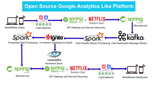
Here is the High Level architecture of the Google Analytics (GA) like Backend System.

Components Breakdown

Web/Mobile Visitor Tracking Code

Every web page or mobile site tracked by GA embed tracking code that collects data about the visitor. It loads an async script that assigns a tracking cookie to the user if it is not set. It also sends an XHR request for every user interaction.

HAProxy Load Balancer

HAProxy, which stands for High Availability Proxy, is a popular open source software TCP/HTTP Load Balancer and proxying solution. Its most common use is to improve the performance and reliability of a server environment by distributing the workload across multiple servers. It is used in many high-profile environments, including: GitHub, Imgur, Instagram, and Twitter.

A backend can contain one or many servers in it — generally speaking, adding more servers to your backend will increase your potential load capacity by spreading the load over multiple servers. Increased reliability is also achieved through this manner, in case some of your backend servers become unavailable.

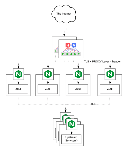
HAProxy routes the requests coming from Web/Mobile Visitor site to the Zuul API Gateway of the solution. Given the nature of a distributed system built for scalability and stateless request and response handling we can distribute the Zuul API gateways spread across geographies. HAProxy performs load balancing (layer 4 + proxy) across our Zuul nodes. High-Availability (HA ) is provided via Keepalived.

Spring Boot & Netflix OSS Eureka + Zuul

Zuul is an API gateway and edge service that proxies requests to multiple backing services. It provides a unified “front door” to the application ecosystem, which allows any browser, mobile app or other user interface to consume services from multiple hosts. Zuul is integrated with other Netflix stack components like Hystrix for fault tolerance and Eureka for service discovery or use it to manage routing rules, filters and load balancing across your system. Most importantly all of those components are well adapted by Spring framework through Spring Boot/Cloud approach.

An API gateway is a layer 7 (HTTP) router that acts as a reverse proxy for upstream services that reside inside your platform. API gateways are typically configured to route traffic based on URI paths and have become especially popular in the microservices world because exposing potentially hundreds of services to the Internet is both a security nightmare and operationally difficult. With an API gateway, one simply exposes and scales a single collection of services (the API gateway) and updates the API gateway’s configuration whenever a new upstream should be exposed externally. In our case Zuul is able to auto discover services registered in Eureka server.

Eureka server acts as a registry and allows all clients to register themselves and used for Service Discovery to be able to find IP address and port of other services if they want to talk to. Eureka server is a client as well. This property is used to setup Eureka in highly available way. We can have Eureka deployed in a highly available way if we can have more instances used in the same pattern.

Spring Boot Microservices

Using a microservices approach to application development can improve resilience and expedite the time to market, but breaking apps into fine-grained services offers complications. With fine-grained services and lightweight protocols, microservices offers increased modularity, making applications easier to develop, test, deploy, and, more importantly, change and maintain. With microservices, the code is broken into independent services that run as separate processes.

Scalability is the key aspect of microservices. Because each service is a separate component, we can scale up a single function or service without having to scale the entire application. Business-critical services can be deployed on multiple servers for increased availability and performance without impacting the performance of other services. Designing for failure is essential. We should be prepared to handle multiple failure issues, such as system downtime, slow service and unexpected responses. Here, load balancing is important. When a failure arises, the troubled service should still run in a degraded functionality without crashing the entire system. Hystrix Circuit-breaker will come into rescue in such failure scenarios.

The microservices are designed for scalability, resilience, fault-tolerance and high availability and importantly it can be achieved through deploying the services in a Docker Swarm or Kubernetes cluster. Distributed and geographically spread Zuul API gateways route requests from web and mobile visitors to the microservices registered in the load balanced Eureka server.

The core processing logic of the backend system is designed for scalability, high availability, resilience and fault-tolerance using distributed Streaming Processing, the microservices will ingest data to Kafka Streams data pipeline.

Apache Kafka Streams

Apache Kafka is used for building real-time streaming data pipelines that reliably get data between many independent systems or applications.

It allows:

Publishing and subscribing to streams of records

Storing streams of records in a fault-tolerant, durable way

It provides a unified, high-throughput, low-latency, horizontally scalable platform that is used in production in thousands of companies.

Kafka Streams being scalable, highly available and fault-tolerant, and providing the streams functionality (transformations / stateful transformations) are what we need — not to mention Kafka being a reliable and mature messaging system.

Kafka is run as a cluster on one or more servers that can span multiple datacenters spread across geographies. Those servers are usually called brokers.

Kafka uses Zookeeper to store metadata about brokers, topics and partitions.

Kafka Streams is a pretty fast, lightweight stream processing solution that works best if all of the data ingestion is coming through Apache Kafka. The ingested data is read directly from Kafka by Apache Spark for stream processing and creates Timeseries Ignite RDD (Resilient Distributed Datasets).

Apache Spark

Spark Streaming is an extension of the core Spark API that enables scalable, high-throughput, fault-tolerant stream processing of live data streams.

It provides a high-level abstraction called a discretized stream, or DStream, which represents a continuous stream of data.

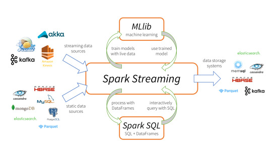
DStreams can be created either from input data streams from sources such as Kafka, Flume, and Kinesis, or by applying high-level operations on other DStreams. Internally, a DStream is represented as a sequence of RDDs (Resilient Distributed Datasets).

Apache Spark is a perfect choice in our case. This is because Spark achieves high performance for both batch and streaming data, using a state-of-the-art DAG scheduler, a query optimizer, and a physical execution engine.

In our scenario Spark streaming process Kafka data streams; create and share Ignite RDDs across Apache Ignite which is a distributed memory-centric database and caching platform.

Apache Ignite

Apache Ignite is a distributed memory-centric database and caching platform that is used by Apache Spark users to:

Achieve true in-memory performance at scale and avoid data movement from a data source to Spark workers and applications.

More easily share state and data among Spark jobs.

Apache Ignite is designed for transactional, analytical, and streaming workloads, delivering in-memory performance at scale. Apache Ignite provides an implementation of the Spark RDD which allows any data and state to be shared in memory as RDDs across Spark jobs. The Ignite RDD provides a shared, mutable view of the same data in-memory in Ignite across different Spark jobs, workers, or applications.

The way an Ignite RDD is implemented is as a view over a distributed Ignite table (aka. cache). It can be deployed with an Ignite node either within the Spark job executing process, on a Spark worker, or in a separate Ignite cluster. It means that depending on the chosen deployment mode the shared state may either exist only during the lifespan of a Spark application (embedded mode), or it may out-survive the Spark application (standalone mode).

With Ignite, Spark users can configure primary and secondary indexes that can bring up to 1000x performance gains.

Apache Cassandra

We will use Apache Cassandra as storage for persistence writes from Ignite.

Apache Cassandra is a highly scalable and available distributed database that facilitates and allows storing and managing high velocity structured data across multiple commodity servers without a single point of failure.

The Apache Cassandra is an extremely powerful open source distributed database system that works extremely well to handle huge volumes of records spread across multiple commodity servers. It can be easily scaled to meet sudden increase in demand, by deploying multi-node Cassandra clusters, meets high availability requirements, and there is no single point of failure.

Apache Cassandra has best write and read performance.

Characteristics of Cassandra:

It is a column-oriented database

Highly consistent, fault-tolerant, and scalable

The data model is based on Google Bigtable

The distributed design is based on Amazon Dynamo

Right off the top Cassandra does not use B-Trees to store data. Instead it uses Log Structured Merge Trees (LSM-Trees) to store its data. This data structure is very good for high write volumes, turning updates and deletes into new writes.

In our scenario we will configure Ignite to work in write-behind mode: normally, a cache write involves putting data in memory, and writing the same into the persistence source, so there will be 1-to-1 mapping between cache writes and persistence writes. With the write-behind mode, Ignite instead will batch the writes and execute them regularly at the specified frequency. This is aimed at limiting the amount of communication overhead between Ignite and the persistent store, and really makes a lot of sense if the data being written rapidly changes.

Analytics Dashboard

Since we are talking about scalability, high availability, resilience and fault-tolerance, our analytics dashboard backend should be designed in a pretty similar way we have designed the web/mobile visitor backend solution using HAProxy Load Balancer, Zuul API Gateway, Eureka Service Discovery and Spring Boot Microservices.

The requests will be routed from Analytics dashboard through microservices. Apache Spark will do processing of time series data shared in Apache Ignite as Ignite RDDs and the results will be sent across to the dashboard for visualization through microservices

0 notes

abhilashkrish · 5 years

Text

Blaze Language and Virtual Machine

I had been quite busy with so many things in the past few years hence I was unable to complete few of the projects which I had started in the past.

Now I am finding leeway to squeeze some time to allot for open source projects which I have started in the past. And the one which excites me most is Blaze Programming Language and Virtual Machine.

Blaze project aims to be a General Purpose Programming Language and Virtual Machine for Multi-Core Processors and General Purpose GPU (GPGPU) Computing.

Blaze Language will be a compiled and interpreted programming language. Blaze will follow the philosophy of Java, "Write once, run anywhere" (WORA). Blaze Compiler will compile and generate Blaze Bytecode (Intermediate Language Representation) in Blaze Class file. Blaze VM will interpret and execute the Class file containing Bytecode at runtime. Blaze VM will be a Stack based Virtual Machine implementation written in C++ 17 standards.

I have made few commits into the GitHub repository of Blaze project. You are invited to follow the project on GitHub

Any comments or suggestions are welcome.

0 notes

abhilashkrish · 5 years

Text

HashMap implementation in Java

HashMap is a data structure to store key-value pairs. We are going to implement a HashMap in Java using Generics. This implementation is based on an array of Entry objects. Entry object stores key and value of the entry to be added in the HashMap.

HashMap uses O(1) time complexity for store and retrieve operations. HashMap internally uses a hash function to calculate the slot to store and retrieve the entry in the array in constant time.

The hash value to locate the slot in the array is calculated using the following method:

(hashcode(key) & 0x7fffffff) % size

AND operation is a shift mask to take care of negative value of hashcode of the key.

There are quite a few other ways to locate the slots such as folding method, mid-squared method etc.

For this implementation we calculate the hash by taking the modulus of the resultant value from hashcode of the key and shift masking with the size of the array.

When two entries hash to the same slot in the array it is called collission. There are quite a few ways we can handle collission resolution such as Separate Chaining (Open Hashing), Linear Probing (Open Addressing or Closed Hashing). At the moment we can skip it for simplicity.

Let's dive into the implementation.

import java.util.Arrays; import java.util.Optional; public class HashMap<K, V> { private int initialCapacity; private int size; private float loadFactor; private Entry<K, V> entries[]; public HashMap() { this.initialCapacity = 20; this.loadFactor = 0.75f; this.size = initialCapacity; this.entries = new Entry[size]; } public HashMap(int initialCapacity) { this.initialCapacity = initialCapacity; this.loadFactor = 0.75f; this.size = initialCapacity; this.entries = new Entry[size]; } public HashMap(int initialCapacity, float loadFactor) { this.initialCapacity = initialCapacity; this.loadFactor = loadFactor; this.size = initialCapacity; this.entries = new Entry[size]; } public int size() { return this.size; } private int hash(K key) { int h = key.hashCode() & 0x7fffffff; return h % size; } public Optional<V> get(K key) { int index = hash(key); if (index >= size) return Optional.empty(); return Optional.of(entries[index].getValue()); } public void put(K key, V value) { int index = hash(key); if (index >= size) resize(index); this.entries[index] = new Entry(key, value); } private void resize(int index) { int newSize = size + (int)(size * loadFactor); if (newSize < index) newSize += index; this.entries = Arrays.copyOf(entries, newSize); this.size = newSize; } public boolean containsKey(K key) { int index = hash(key); if (entries[index] != null && entries[index].getKey().equals(key)) return true; return false; } private static class Entry<K, V> { private K key; private V value; private Entry() { } public Entry(K key, V value) { this.key = key; this.value = value; } public K getKey() { return key; } public void setKey(K key) { this.key = key; } public V getValue() { return value; } public void setValue(V value) { this.value = value; } } }

Let's test the HashMap implementation. I got this simple problem from a Fintech company where they get Bank Account numbers of customers in different formats sometimes masked. The problem is like they have a set of raw Bank Account numbers and the corresponding processed Bank Account Numbers available with the system. They have to do pattern matching of the Bank Account numbers coming into the system with the best possible match in O(1) time complexity. There can be scenario where they process the Bank Account number of same customer more than once. HashMap is one of the best fits for this scenario. In a production deployment using any caching solution is the way to go.

public class Main { private HashMap<String, String> map = new HashMap<>(); public static void main(String args[]) { Main main = new Main(); main.addTextToMap("12345678", "0012345678"); main.addTextToMap("1235xx78", "0012345678"); main.addTextToMap("0015678", "0015678"); main.addTextToMap("345678", "345678"); main.addTextToMap("0012345678", "0012345678"); String textToMatch = "1235xx78"; System.out.println("Input: " + textToMatch); if (main.match(textToMatch)) { System.out.println("Text is matched"); System.out.println("Output: " + main.getTextFromHashMap(textToMatch)); } } private String getTextFromHashMap(String input) { return map.get(input).get(); } private void addTextToMap(String input, String output) { map.put(input, output); } private boolean match(String text) { boolean flag = false; if (map.containsKey(text)) flag = true; return flag; } }

0 notes

abhilashkrish · 5 years

Text

Kafka as Enterprise Service Bus [Scala]

We are modelling a system where customer consults stock price. We are using Apache Kafka as Enterprise Service Bus (ESB) which acts as the middleware.

Enterprise Service Bus (ESB) consists of taking one or more events from an event stream and applying actions over those events. The most common actions performed by ESB are:

Data Transformation

Event Handling

Protocol Conversion

Data Mapping

In our example we are performing Event Modelling through Apache Kafka as ESB.

The first step in the event modellling is to express the event in English in the following form:

Subject-verb-direct object

For this example we are modelling the event customer consults stock price

The subject in the sentence is customer

The verb in the sentence is consults

The direct object in the sentence is stock price

We represent our message in JSON format.

The sample message in JSON format is,

{ "event": "CUSTOMER_CONSULTS_STOCKPRICE", "customer": { "id": "13548310", "name": "Abhilash, Krishnan", "ipAddress": "185.86.151.11" }, "stock": { "name": "GOOG", "price": "USD" }, "timestamp": "2018-09-28T08:08:14Z" }

In our example we have Readers or Consumers, Writers or Producers and a Processing Engine.

The process flow can be depicted as:

Kafka Producer Console -> input-topic

Reader or Consumer <- input-topic

Process the received message

Writer or Producer -> output-topic

Kafka Consumer Console <- output-topic

Now let's develop the Scala application to receive messages from Kafka Producer Console and process the messages and write the messages to Kafka Consumer Console.

import java.util.Properties trait Consumer { def createConfig(servers: String): Properties def run(producer: Producer): Unit }

import java.time.Duration import java.util.{Collections, Properties} import org.apache.kafka.clients.consumer.{ConsumerRecord, ConsumerRecords, KafkaConsumer} class Reader(servers: String, groupId: String, topic: String) extends Consumer { val consumer: KafkaConsumer[String,String] = new KafkaConsumer[String, String](createConfig(servers)) override def createConfig(servers: String): Properties = { val config = new Properties(); config.setProperty("bootstrap.servers", servers) config.setProperty("group.id", groupId) config.setProperty("enable.auto.commit", "true") config.setProperty("auto.commit.interval.ms", "1000") config.setProperty("auto.offset.reset", "earliest") config.setProperty("session.timeout.ms", "30000") config.setProperty("key.deserializer", "org.apache.kafka.common.serialization.StringDeserializer") config.setProperty("value.deserializer", "org.apache.kafka.common.serialization.StringDeserializer") config } override def run(producer: Producer): Unit = { this.consumer.subscribe(Collections.singletonList(this.topic)) while (true) { val records: ConsumerRecords[String, String] = consumer.poll(Duration.ofMillis(100)) records.forEach( record => { println("Read record value " + record.value() + " from topic " + topic) producer.process(record.value()) }) } } }

import java.util.Properties trait Producer { def createConfig(servers: String): Properties def process(message: String) def write(message: String) }

import java.util.Properties import org.apache.kafka.clients.producer.{KafkaProducer, ProducerRecord} class Writer(servers: String, topic: String) extends Producer { val producer: KafkaProducer[String, String] = new KafkaProducer[String, String](createConfig(servers)) override def createConfig(servers: String): Properties = { val config = new Properties() config.setProperty("bootstrap.servers", servers) config.setProperty("acks", "all") config.setProperty("retries", "0") config.setProperty("batch.size", "1000") config.setProperty("linger.ms", "1") config.setProperty("key.serializer", "org.apache.kafka.common.serialization.StringSerializer") config.setProperty("value.serializer", "org.apache.kafka.common.serialization.StringSerializer") config } override def process(message: String): Unit = { write(message) } override def write(message: String): Unit = { val record = new ProducerRecord[String, String](topic, message) producer.send(record) println("Write Message: " + message + " to topic " + topic) } }

object ProcessingEngine { def main(args: Array[String]): Unit = { val servers: String = "localhost:9093" val groupId: String = "stock" val sourceTopic: String = "input-topic" val targetTopic: String = "output-topic" val reader: Reader = new Reader(servers, groupId, sourceTopic) val writer: Writer = new Writer(servers, targetTopic) reader.run(writer) } }

To run this application do the following steps:

Start Zookeeper with the following command:

zookeeper-server.sh zookeeper.properties

Minimal zookeeper.properties file entries are,

# the directory where the snapshot is stored. dataDir=/kafka/zookeeper # the port at which the clients will connect clientPort=2181 # disable the per-ip limit on the number of connections since this is a non-production config maxClientCnxns=0

Start Kafka broker instance running on localhost at port 9093 with the following command:

kafka-server-start.sh server.properties

Minimal server.properties file entries are,

broker.id=1 port=9093 zookeeper.connect=localhost:2181 log.dirs=/tmp/kafka/server-1-logs offsets.topic.replication.factor=1

Start Kafka Producer console

kafka-console-producer.sh --broker-list localhost:9093 --topic input-topic

Start Kafka Consumer console

kafka-console-consumer.sh --bootstrap-server localhost:9093 --topic output-topic

Run the Scala application we have developed.

Send the following JSON message from Kafka Producer console opened in Step 3.

You will be able to see the JSON message in the Kafka Consumer console opened in Step 4.

In the next set of tutorials I will be explaing more on how we can validate the data, enrichment of messages, extracting the data, write custom serializer etc.

0 notes

abhilashkrish · 5 years

Text

N-Queens Problem (Backtracking)

The N-Queens is the problem of placing N chess queens on an N×N chessboard so that no two queens attack each other. In chess, a queen can move as far as she pleases, horizontally, vertically, or diagonally.

A chess board has 8 rows and 8 columns. The standard 8 by 8 Queens' problem asks how to place 8 queens on an ordinary chess board so that none of them can hit any other in one move.

Here is the solution for 4x4 chessboard.

Solution:

Create a solution matrix of the same structure as chess board.

Whenever a queen is placed on the chess board, mark that particular cell in solution matrix.

At the end print the solution matrix, the marked cells will show the positions of the queens on the chess board.

public class NQueens { private int solution[][]; public NQueens(int n) { solution = new int[n][n]; for (int row = 0; row < n; row++) { for (int col = 0; col < n; col++) { solution[row][col] = 0; } } } public static void main(String args[]) { NQueens nQueens = new NQueens(4); nQueens.solveFor(4); } public void solveFor(int n) { if (placeQueens(0, n)) { for (int i = 0; i < n; i++) { for (int j = 0; j < n; j++) { System.out.print(" " + solution[i][j]); } System.out.println(" "); } } } private boolean placeQueens(int queen, int n) { //We have found solution if (queen == n) return true; for ( int row = 0; row < n; row++) { //Check if queen can be placed if (canPlace(solution, row, queen)) { //Place the queen solution[row][queen] = 1; //solve for next queen if (placeQueens(queen+1, n)) return true; //Above placement didn't work //Backtrack solution[row][queen] = 0; } } return false; } private boolean canPlace(int matrix[][], int row, int col) { //Check the row for (int i = 0; i < col; i++) { if (matrix[row][i] == 1) return false; } //Check the upper diagonal for (int i = row, j = col; i >=0 && j >= 0; i--, j--) { if (matrix[i][j] == 1) return false; } //Check the lower diagonal for (int i = row, j = col; i < matrix.length && j >= 0; i++, j--) { if (matrix[i][j] == 1) return false; } return true; } }

0 notes

abhilashkrish · 5 years

Text

Towers of Hanoi Puzzle

The Towers of Hanoi is a mathematical puzzle. It consists of three rods (or pegs or towers) and a number of disks of different sizes which can slide onto any rod. The puzzle starts with the disks on one rod in ascending order of size, the smallest at the top, thus making a conical shape.

The objective of the puzzle is to move the entire stack to another rod, satisfying the following rules:

Only one disk may be moved at a time.

Each move consists of taking the upper disk from one of the rods and sliding it onto another rod, on top of the other disks that may already be present on that rod.

No disk may be placed on top of a smaller disk.

Algorithm

Move the top n – 1 disks from Source to Auxiliary tower.

Move the nth disk from Source to Destination tower.

Move the n – 1 disks from Auxiliary tower to Destination tower.

Transferring the top n – 1 disks from Source to Auxiliary tower can again be thought of as a fresh problem and can be solved in the same manner.

Let's dive into the solution using Python.

class TowersOfHanoi: def move_disk(self, n, f, to, aux): if n == 1: print('Disk moved from ' + f + ' to ' + to) return #Move top n-1 disks from A to B with C as auxillary self.move_disk(n-1, f, aux, to) #Move remaining disks from A to C print('Disk moved from ' + f + ' to ' + to) #Move n-1 disks from B to C with A as auxillary self.move_disk(n-1, aux, to, f) def main(): toh = TowersOfHanoi() n = 3 toh.move_disk(n, 'A', 'C', 'B') if __name__ == "__main__": main()

0 notes

abhilashkrish · 5 years

Text

Find the number of elements in a given range

In a Binary Search Tree (BST) find the number of elements in a given range.

class Node: def __init__(self, data, left, right): self.data = data self.left = left self.right = right class Solution: def create_tree(self): left = Node(1, None, None) right = Node(3, None, None) root = Node(2, left, right) return root def range_check(self, node, start, end): if node is None: return 0 if (node.data > start) and (node.data < end): return 1 + self.range_check(node.left, start, end) + self.range_check(node.right, start, end) elif node.data >= end: return self.range_check(node.left, start, end) else: return self.range_check(node.right, start, end) def main(): sol = Solution() tree = sol.create_tree() nodes = sol.range_check(tree, 0, 4) print("Number of nodes are {}".format(nodes)) if __name__ == "__main__": main()

0 notes

abhilashkrish · 5 years

Text

Find the majority element

In this problem, majority element is defined as the number that appears more than n/2 times in an array of numbers.

class Solution: def __init__(self, nums): self.nums = nums def find_majority(self): majority = self.nums[0] count = 0 for num in self.nums: if num == majority: count += 1 else: count -= 1 if count == 0: majority = num count = 1 return majority def verify_majority(self, majority): count = 0 n = len(self.nums) for num in self.nums: if num == majority: count += 1 if count > n/2: return True return False def main(): nums = [1, 1, 2, 3, 3, 3, 4, 5, 5, 5, 5, 5, 5, 5, 5, 5, 5] solution = Solution(nums) majority = solution.find_majority() if solution.verify_majority(majority): print("Majority is {}".format(majority)) else: print("No majority found") if __name__ == "__main__": main()

0 notes

abhilashkrish · 5 years

Text

Linear Regression using scikit-learn

Predicting the number of marks a student will score in a test depending on the number of hours they have studied for the test.

import numpy as np import pandas as pd dataset = pd.read_csv('student_marks.csv') X=dataset.iloc[:,:-1].values y=dataset.iloc[:,1].values from sklearn.model_selection import train_test_split X_train,X_test,y_train,y_test = train_test_split(X,y,test_size=0.2,random_state=0) from sklearn.linear_model import LinearRegression linear_regression = LinearRegression() linear_regression.fit(X_train,y_train) pred_y=linear_regression.predict(X_test) df=pd.DataFrame({'Actual':y_test, 'Predicted':pred_y}) print(df) from sklearn import metrics print('MEAN ABSOLUTE ERROR: ',metrics.mean_absolute_error(y_test,pred_y)) print('MEAN SQUARED ERROR: ',metrics.mean_squared_error(y_test,pred_y)) print('ROOT MEAN SQUARED ERROR: ',np.sqrt(metrics.mean_squared_error(y_test,pred_y)))

You can use the following data in the student_marks.csv

Hours,Marks 2.1,21 5.1,47 3.2,27 8.5,75 3.5,30 1.5,18 4.3,39 3.8,32 5.5,50 1.8,19 4.5,42 4.7,46

0 notes

abhilashkrish · 5 years

Text

Rotate Array

Rotate an array of size ‘n’ by ‘d’ elements.

#include <stdio.h> void rotateByOne(int arr[], int n) { int temp = arr[0]; int i; for (i = 0; i < n-1; i++) arr[i] = arr[i+1]; arr[i] = temp; } void rotate(int arr[], int n, int d) { for (int i = 0; i < d; i++) rotateByOne(arr, n); } void printArray(int arr[], int n) { for (int i = 0; i < n; i++) printf(" %d ", arr[i]); } int main() { int arr[] = {1, 2, 3, 4}; rotate(arr, 4, 2); printArray(arr, 4); return 0; }

0 notes

abhilashkrish · 6 years

Text

Akka Actor System

Akka is an open source toolkit from Lightbend to create production-ready concurrent, distributed and fault-tolerant applications.

Akka is Scala’s implementation of an Actor concurrency model made popular in part by Erlang. To use Akka, you define a set of workers (Actors) that listen for messages in a mailbox and act on them in some way.

Akka can also be set up as a distributed system, where actors can run across any number of machines, not just within your local JVM. This means message passing happens over a remote RPC call rather than an internal function call, but the complexity is entirely handled by the Akka runtime.

For starters, let’s write a simple Akka Actor example. It's a conversation in French with the Akka Actor.

import akka.actor.Actor import akka.actor.Props import akka.actor.ActorSystem class GreetActor extends Actor { def receive = { case "Bonjour" => println("Bonjour, Quoi de neuf?") case _ => println("Au revoir!") } } object Main extends App { val system = ActorSystem("GreetActorSystem") val greetactor = system.actorOf(Props[GreetActor], name = "greetactor") greetactor ! "Bonjour" greetactor ! "Ciao!" }

We need an ActorSystem to set the ball rolling.

val system = ActorSystem("GreetActorSystem")

ActorSystem is created in the above code snippet with an arbitary string.

val greetactor = system.actorOf(Props[GreetActor], name = "greetactor")

In the above code snippet we have created an Actor instance with actorOf, and that line shows the syntax for an Actor whose default constructor takes no arguments.

Now we can send messages to the actor instance with the below lines.

greetactor ! "Bonjour" greetactor ! "Ciao!"

More complex examples of Akka Actor System in upcoming posts.

0 notes

abhilashkrish · 6 years

Text

Tensors in Python

Tensors are a type of data structure used in linear algebra, and like vectors and matrices, you can calculate arithmetic operations with tensors.

A tensor is a generalization of vectors and matrices and is easily understood as a multidimensional array.

A vector is a one-dimensional or first order tensor and a matrix is a two-dimensional or second order tensor.

Tensor representation in Python

Like vectors and matrices, tensors can be represented in Python using the N-dimensional array (ndarray).

A tensor can be defined in-line to the constructor of array() as a list of lists.

Let's get our hands dirty by creating a tensor in Python using NumPy ndarray. The example below defines 3x3x3 tensor.

from numpy import array T = array([ [[1, 2,3], [4, 5, 6], [7, 8, 9]], [[10, 11, 12], [13, 14, 15], [16, 17, 18]], [[20, 21, 22], [23, 24, 25], [26, 27, 28]] ]) print(T.shape) print(T)

Running the code first prints the shape of the tensor (3, 3, 3), then the values of the tensor itself. The tensor is printed as a series of matrices, one for each layer.

[[[ 1 2 3] [ 4 5 6] [ 7 8 9]] [[10 11 12] [13 14 15] [16 17 18]] [[20 21 22] [23 24 25] [26 27 28]]]

For this 3D tensor, axis 0 specifies the level, axis 1 specifies the column, and axis 2 specifies the row.

Tensor Addition

The addition of two tensors of the same dimension results in a new tensor of the same dimension. Each scalar value is the addition of the scalar values in the parent tensors.

from numpy import array A = array([ [[1, 2, 3], [4, 5, 6], [7, 8, 9]], [[10, 11, 12], [13, 14, 15], [16, 17, 18]], [[20, 21, 22], [23, 24, 25], [26, 27, 28]] ]) B = array([ [[1, 2, 3], [4, 5, 6], [7, 8, 9]], [[10, 11, 12], [13, 14, 15], [16, 17, 18]], [[20, 21, 22], [23, 24, 25], [26, 27, 28]] ]) C = A + B print(C)

Running the above code results in the addition of tensors A and B.

[[[ 2 4 6] [ 8 10 12] [14 16 18]] [[20 22 24] [26 28 30] [32 34 36]] [[40 42 44] [46 48 50] [52 54 56]]]

Tensor Subtraction

The subtraction of two tensors of the same dimension results in a new tensor of the same dimension. Each scalar value is the substraction of the scalar values in the parent tensors.

Running the above code results in the subtraction of tensors A and B.

[[[0 0 0] [0 0 0] [0 0 0]] [[0 0 0] [0 0 0] [0 0 0]] [[0 0 0] [0 0 0] [0 0 0]]]

Tensor Hadamard Product

The element-wise multiplcation of two tensors of the same dimension results in a new tensor of the same dimension. Each scalar value is the multiplication of the scalar values in the parent tensors.

As with matrices, the operation is referred to as the Hadamard Product to differentiate it from tensor multiplication.

Running the above code results in the multiplication of tensors A and B.

[[[ 1 4 9] [ 16 25 36] [ 49 64 81]] [[100 121 144] [169 196 225] [256 289 324]] [[400 441 484] [529 576 625] [676 729 784]]]

Tensor Division

The divsion of two tensors of the same dimension results in a new tensor of the same dimension. Each scalar value is the divison of the scalar values in the parent tensors.

Running the above code results in the divsion of tensors A and B.

[[[1. 1. 1.] [1. 1. 1.] [1. 1. 1.]] [[1. 1. 1.] [1. 1. 1.] [1. 1. 1.]] [[1. 1. 1.] [1. 1. 1.] [1. 1. 1.]]]

Tensor Product

Tensor A with q dimensions and tensor B with r dimensions, the product of these tensors will be a new tensor with the order of q + r or, said another way, q + r dimensions.

The tensor product can be implemented in NumPy using the tensordot() function.

The function takes as arguments the two tensors to be multiplied and the axis on which to sum the products over, called the sum reduction. To calculate the tensor product, also called the tensor dot product in NumPy, the axis must be set to 0.

In the code below we define two order-1 tensors (vectors) and calculate the tensor product.

from numpy import array from numpy import tensordot A = array([1, 2]) B = array([3, 4]) C = tensordot(A, B, 0) print(C)

Running the above code results in the tensor product of A and B.

[[3 4] [6 8]]

0 notes

abhilashkrish · 6 years

Text

Plunge into Big Data with Apache Spark and Scala

As a part of a series of tutorials on Big Data with Apache Spark and Scala let’s dive into the first part of the series.

The objective of the tutorial is to count the number of lines containing ‘a’s and ‘b’s in a big text file.

Let’s write the program and explain it step by step.

import org.apache.spark.SparkConf import org.apache.spark.SparkContext import org.apache.spark.SparkContext._ object CountLines { def main(args: Array[String]) { val bigFile = "/somebigtextfile" val host = "LocalHost" val conf = new SparkConf().setAppName("First Spark App").setMaster("local[2]"). set("spark.driver.host",host).set("spark.driver.port","8080") val sc = new SparkContext(conf) val bigData = sc.textFile(bigFile, 2).cache() val numAs = bigData.filter(line => line.contains("a")).count() val numBs = bigData.filter(line => line.contains("b")).count() println("Lines with a: %s, Lines with b: %s".format(numAs, numBs)) } }

Running Spark applications on Windows in general is no different than running it on other operating systems like Linux or macOS.

What makes the huge difference between the operating systems is Hadoop that is used internally for file system access in Spark.

You may run into few minor issues when you are on Windows due to the way Hadoop works with Windows' POSIX-incompatible NTFS filesystem. Download winutils.exe binary from http://public-repo-1.hortonworks.com/hdp-win-alpha/winutils.exe

Save winutils.exe binary to a directory of your choice, e.g. C:\hadoop\bin.

Set HADOOP_HOME to reflect the directory with winutils.exe (without bin).

val bigFile = "/somebigtextfile" val host = "LocalHost"

Specify the location of the big text file and host machine in this case LocalHost.

val conf = new SparkConf().setAppName("First Spark App").setMaster("local[2]"). set("spark.driver.host",host).set("spark.driver.port","8080")

Spark properties control most application settings and are configured separately for each application. These properties can be set directly on a SparkConf passed to your SparkContext. SparkConf allows you to configure some of the common properties (e.g. master URL and application name), as well as arbitrary key-value pairs through the set() method.

Note that we run with local[2], meaning two threads - which represents “minimal” parallelism, which can help detect bugs that only exist when we run in a distributed context.

The spark driver is the program that declares the transformations and actions on RDDs of data and submits such requests to the master. In practical terms, the driver is the program that creates the SparkContext, connecting to a given Spark Master.

val sc = new SparkContext(conf)

SparkContext (aka Spark context) is the heart of a Spark application. SparkContext is created by passing SparkConf. Spark context sets up internal services and establishes a connection to a Spark execution environment. Once a SparkContext is created you can use it to create RDDs, accumulators and broadcast variables, access Spark services and run jobs (until SparkContext is stopped). A Spark context is essentially a client of Spark’s execution environment and acts as the master of your Spark application (don’t get confused with the other meaning of Master in Spark, though).

val bigData = sc.textFile(bigFile, 2).cache()

SparkContext creates RDD (Resilient Distributed Dataset) with 2 partitions from the text file and stores it in memory.

RDD (Resilient Distributed Dataset) is a collection of elements, that can be divided across multiple nodes in a cluster for parallel processing. It is also fault tolerant collection of elements, which means it can automatically recover from failures. RDD is immutable, we can create RDD once but can’t change it.

A partition (aka split) is a logical chunk of a large distributed data set.

val numAs = bigData.filter(line => line.contains("a")).count() val numBs = bigData.filter(line => line.contains("b")).count() println("Lines with a: %s, Lines with b: %s".format(numAs, numBs))

Count the lines containing 'a's and 'b's by applying filter action of RDD and print the count of lines with 'a's and 'b's.

More tutorials on Big Data with Apache Spark and Scala in the upcoming series.

0 notes